Module 3
Understand: Understanding Data and Data Structures
Overview
Summary
Importing data successfully doesn’t mean that we have all the information about our data. Understanding data structures and variable types in the data set are also crucial for conducting data preprocessing. We shouldn’t be performing any type of data preprocessing without understanding what we have in hand. In this module, I will provide the basics of variable types and data structures. You will learn to check the types of the variables, dimensions and structure of the data, and levels/values for the variables. We will also cover how to manipulate the format of the data (i.e., data type conversions). Finally, the difference between wide and long formatted data will be explained.
Learning Objectives
The learning objectives of this module are as follows:
- Understand R’s basic data types (i.e., character, numeric, integer, factor, and logical).
- Understand R’s basic data structures (i.e., vector, list, matrix, and data frame) and main differences between them.
- Learn to check attributes (i.e., name, dimension, class, levels etc.) of R objects.
- Learn how to convert between data types/structures.
- Understand the difference between wide vs. long formatted data.
Types of variables
A data set is a collection of measurements or records which are often called as variables and there are two major types of variables that can be stored in a data set: qualitative and quantitative. The qualitative variable is often called as categorical and they have a non-numeric structure such as gender, hair colour, type of a disease, etc. The qualitative variable can be nominal or ordinal.
Nominal variable: They have a scale in which the numbers or letters assigned to objects serve as labels for identification or classification. Examples of this variable include binary variables (e.g., yes/no, male/female) and multinomial variables (e.g. religious affiliation, eye colour, ethnicity, suburb).
Ordinal variable: They have a scale that arranges objects or alternatives according to their ranking. Examples include the exam grades (i.e., HD, DI, Credit, Pass, Fail etc.) and the disease severity (i.e., severe, moderate, mild).
The second type of variable is called the quantitative variable. These variables are the numerical data that we can either measure or count. The quantitative variables can be either discrete or continuous.
Continuous quantitative variable: They arise from a measurement process. Continuous variables are measured on a continuum or scale. They can have almost any numeric value and can be meaningfully subdivided into finer and finer increments, depending upon the precision of the measurement system. For example: time, temperature, wind speed may be considered as continuous quantitative variables.
Discrete quantitative variable: They arise from a counting process. Examples include the number of text messages you sent this past week and the number of faults in a manufacturing process.
The following short video by Nicola Petty provides a great overview
on the variable types. Note that, in some statistical sources, the “type
of the data” and the “type of the variables” are used synonymously. In
the following video, the term “types of data” are used
to refer the “types of variables”.
Data Types in R
In the previous section, we defined the types of variables in a general sense. However, as R is a programming language it has own definitions of data types and structures. Technically, R classifies all the different types of data into four classes:
- Logical: This class consists of TRUE or FALSE (binary) values. A logical value is often created via comparison between variables.
x <- 10
y <- (x > 0)
y
## [1] TRUEWe can use class() function to check the class of an
object.
# check the class of y

class(y)
## [1] "logical"- Numeric (integer or double): Quantitative values
are called as numeric in R. It is the default computational data type.
Numeric class can be integer or double. Integer types can be seen as
discrete values (e.g., 2) whereas, double class will have floating point
numbers (e.g., 2.16).
Here is an example of a double numeric variable:
# create a double-precision numeric variable

dbl_var <- c(4, 7.5, 14.5)

# check the class of dbl_var

class(dbl_var)
## [1] "numeric"To check whether a numeric object is integer or double, you can also
use typeof().
# check the type of dbl_var object

typeof(dbl_var)
## [1] "double"In order to create an integer variable, we must place an
L directly after each number. Here is an example:
# create an integer (numeric) variable

int_var <- c(4L, 7L, 14L)

# check the class of int_var

class(int_var)
## [1] "integer"- Character: A character class is used to represent
string values in R. The most basic way to generate a character object is
to use quotation marks
" "and assign a string/text to an object.
# create a character variable using " " and check its class

char_var <- c("debit", "credit", "Paypal")

class(char_var)
## [1] "character"- Factor: Factor class is used to represent
qualitative data in R. Factors can be ordered or unordered. Factors
store the nominal values as a vector of integers in the range [\(1\ldots k\)] (where \(k\) is the number of unique values in the
nominal variable), and an internal vector of character strings (the
original values) mapped to these integers.
Factor objects can be created with the factor()
function:
# create a factor variable using factor()

fac_var1 <- factor( c("Male", "Female", "Male", "Male") )
fac_var1
## [1] Male Female Male Male
## Levels: Female Male# check its class
class(fac_var1)## [1] "factor"To see the levels of a factor object levels() function
will be used:
# check the factor levels

levels(fac_var1)
## [1] "Female" "Male"By default, the levels of the factors will be ordered alphabetically.
Using the levels() argument, we can control the ordering of
the levels while creating a factor:
# create a factor variable using factor() and order the levels using levels() argument

fac_var2 <- factor( c("Male", "Female", "Male", "Male"),
                    levels = c("Male", "Female") )
fac_var2
## [1] Male Female Male Male
## Levels: Male Female# check its levels
levels(fac_var2)## [1] "Male" "Female"We can also create ordinal factors in a specific order using the
ordered = TRUE argument:
# create a ordered factor variable using factor() and order the levels using levels() argument

ordered_fac <-factor( c("DI", "HD", "PA", "NN", "CR", "DI", "HD", "PA"),
                      levels = c("NN", "PA", "CR", "DI", "HD"), ordered=TRUE )

ordered_fac
## [1] DI HD PA NN CR DI HD PA
## Levels: NN < PA < CR < DI < HDThe ordering will be reflected as
NN < PA < CR < DI < HD in the output.
Factors are also created during the data import. Many import
functions like read.csv(), read_cvs(),
read.table() etc. have stringsAsFactors option
that determines how the character data is read in R. For BaseR
read.csv() function, the default setting is
stringsAsFactors = False. However, if we set it to TRUE,
then all columns that are detected to be character/strings are converted
to factor variables.
Let’s read the VIC_pet.csv dataset
available under data repository using read.csv():
pets <- read.csv("data/VIC_pet.csv",stringsAsFactors = TRUE)
head(pets)
## id State Region Animal_Type
## 1 17819v Victoria Colac Otway Dog
## 2 142785v Victoria Wyndham Cat
## 3 97268v Victoria Ballarat Cat
## 4 46906v Victoria Geelong Dog
## 5 35939v Victoria Geelong Dog
## 6 114898v Victoria Ballarat Dog
## Animal_Name
## 1 CHUBBY
## 2
## 3 Bailey
## 4 Shuko
## 5 Violet
## 6 Ralph
## Breed_Description Colour Animal_Desexed
## 1 Labrador NULL
## 2 Domestic
## 3 Burmese
## 4 German Shepherd
## 5 Labrador/Staffordshire
## 6 German Wire Hair Pointerstr(pets)## 'data.frame': 40 obs. of 8 variables:
## $ id : Factor w/ 40 levels "10396v","104515v",..: 15 9 39 21 18 4 30 6 14 25 ...
## $ State : Factor w/ 1 level "Victoria": 1 1 1 1 1 1 1 1 1 1 ...
## $ Region : Factor w/ 7 levels "Ballarat","Colac Otway",..: 2 7 1 3 3 1 3 5 7 3 ...
## $ Animal_Type : Factor w/ 7 levels "Cat","Cat ",..: 7 2 1 4 4 4 4 5 6 1 ...
## $ Animal_Name : Factor w/ 28 levels "","Bailey","Blacky",..: 9 1 2 24 28 20 14 1 1 10 ...
## $ Breed_Description: Factor w/ 34 levels "","American Staffordshire Terrier",..: 23 11 6 14 24 16 28 28 2 11 ...
## $ Colour : Factor w/ 3 levels "","NULL","WHI ": 2 1 1 1 1 1 1 1 1 1 ...
## $ Animal_Desexed : Factor w/ 4 levels "","N","y","Y": 1 1 1 1 1 1 1 4 1 1 ...As seen from the str() output, all of the columns in
pets data are read as factors due to containing strings and
the data was imported using read.csv() with the default
option. Now, let’s focus on Animal_Type variable and check
its levels using:
levels(pets$Animal_Type)## [1] "Cat"
## [2] "Cat "
## [3] "dog"
## [4] "Dog"
## [5] "DOG "
## [6] "Dog "
## [7] "Dog "Note that there are in fact two unique levels for the
Animal_Type i.e. dog and cat. However, due to the automatic
conversion of different strings to factors we observe seven different
levels in Animal_Type, namely “Cat”,
“Cat[whitespace]”, “dog”,
“Dog”,“DOG[whitespace]”,
“Dog[whitespace]”,
“Dog[whitespace][whitespace]”. Again, it is a good practice
to read such strings as characters and then apply string manipulations
(which will be covered in Module 8) to standardize all strings to “dog”
and “cat”.
Now let’s look at the levels of id variable which
contains the unique identification number of the pets:
levels(pets$id)## [1] "10396v" "104515v" "110188v" "114898v" "129666v" "13234v" "137135v"
## [8] "141587v" "142785v" "143032v" "151452v" "151569v" "151921v" "154462v"
## [15] "17819v" "1828v" "18714v" "35939v" "3654v" "39333v" "46906v"
## [22] "49872v" "51127v" "54848v" "55483v" "5754v" "61112v" "64560v"
## [29] "66701v" "70244v" "70794v" "7089v" "77361v" "81001v" "84561v"
## [36] "88946v" "92359v" "93485v" "97268v" "97957v"As seen in the above output, there is no need to factorize
id variable as there are 40 observations and 40 different
levels for the id level. Therefore, any factorization of
id variable would be inefficient. For such cases, it is
better to leave this column as character
(stringsAsFactors = FALSE) during the data import.
As mentioned previously, a data set is a collection of measurements or records which can be in any class (i.e., logical, character, numeric, factor, etc.). Typically, data sets contain many variables of different length and type of values.
Data Structures in R
In R, we can store data sets using vectors, lists, matrices and data frames. In R, vectors, lists, matrices, arrays and data frames are called “Data Structures”.
According to Wickham (2019), R’s base
data structures can be organised by their dimensionality (i.e.,
one-dimension, two-dimension, or n-dimension) and whether they’re
homogeneous (i.e., all contents/variables must be of the same type) or
heterogeneous (i.e., the contents/variables can be of different types).
Therefore, there are five data structures given in the following table
(adapted from Advanced R, Wickham
(2019).)
| Dimension | Homogeneous | Heterogeneous |
|---|---|---|
| one-dimension | Atomic vector | List |
| two-dimension | Matrix | Data frame |
| n-dimension | Array | – |
In this section, we won’t cover the multi-dimensional arrays, but we will go into the details of vectors, lists, matrices, and data frames.
Vectors
A vector is the basic structure in R, which consists of
one-dimensional sequence of data elements of the same basic type (i.e.,
integer, double, logical, or character). Vectors are created by
combining multiple elements into one dimensional array using the
c() function. The one-dimensional examples illustrated
previously are considered vectors.
# a double numeric vector

dbl_var <- c(4, 7.5, 14.5)

# an integer vector

int_var <- c(4L, 7L, 14L)

# a logical vector

log_var <- c(T, F, T, T)

# a character vector

char_var <- c("debit", "credit", "Paypal")
All elements of a vector must be the same type, if you attempt to combine different types of elements, they will be coerced to the most flexible type possible. Here are some examples:
# vector of characters and numerics will be coerced to a character vector

ex1 <- c("a", "b", "c", 1, 2, 3)

# check the class of ex1

class(ex1)
## [1] "character"# vector of numerics and logical will be coerced to a numeric vector
ex2 <- c(1, 2, 3, TRUE, FALSE)
# check the class of ex2
class(ex2)## [1] "numeric"# vector of logical and characters will be coerced to a character vector
ex3 <- c(TRUE, FALSE, "a", "b", "c")
# check the class of ex3
class(ex3)## [1] "character"In order to add additional elements to a vector we can use
c() function.
# add two elements (4 and 6) to the ex2 vector

ex4 <- c(ex2, 4, 6)

ex4
## [1] 1 2 3 1 0 4 6To subset a vector, we can use square brackets [ ] with
positive/negative integers, logical values or names. Here are some
examples:
# take the third element in ex4 vector

ex4[3]
## [1] 3# take the first three elements in ex4 vector
ex4[1:3]## [1] 1 2 3# take the first, third, and fifth element
ex4[c(1,3,5)]## [1] 1 3 0# take all elements except first
ex4[-1]## [1] 2 3 1 0 4 6# take all elements less than 3
ex4[ ex4 < 3 ]## [1] 1 2 1 0Lists
A list is an R structure that allows you to combine elements of
different types and lengths. In order to create a list we can use the
list() function.
# create a list using list() function

list1 <- list(1:3, "a", c(TRUE, FALSE, TRUE), c(2.5, 4.2))

# check the class of list1

class(list1)
## [1] "list"To see the detailed structure within an object we can use the
structure function str(), which provides a compact display
of the internal structure of an R object.
# check the structure of the list1 object

str(list1)
## List of 4
## $ : int [1:3] 1 2 3
## $ : chr "a"
## $ : logi [1:3] TRUE FALSE TRUE
## $ : num [1:2] 2.5 4.2Note how each of the four list items above are of different classes (integer, character, logical, and numeric) and different lengths.
In order to add on to lists we can use the append()
function. Let’s add a fifth element to the list1 and store
it as list2:
# add another list c("credit", "debit", "Paypal") on list1

list2 <- append(list1, list(c("credit", "debit", "Paypal")))

# check the structure of the list2 object

str(list2)
## List of 5
## $ : int [1:3] 1 2 3
## $ : chr "a"
## $ : logi [1:3] TRUE FALSE TRUE
## $ : num [1:2] 2.5 4.2
## $ : chr [1:3] "credit" "debit" "Paypal"R objects can also have attributes, which are like metadata for the
object. These metadata can be very useful in that they help to describe
the object. Some examples of R object attributes are:
- names, dimnames
- dimensions (e.g. matrices, arrays)
- class (e.g. integer, numeric)
- length
- other user-defined attributes/metadata
Attributes of an object (if any) can be accessed using the
attributes() function. Let’s check if list2
has any attributes.
attributes(list2)## NULLWe can add names to lists using names() function.
# add names to a pre-existing list

names(list2) <- c ("item1", "item2", "item3", "item4", "item5")

str(list2)
## List of 5
## $ item1: int [1:3] 1 2 3
## $ item2: chr "a"
## $ item3: logi [1:3] TRUE FALSE TRUE
## $ item4: num [1:2] 2.5 4.2
## $ item5: chr [1:3] "credit" "debit" "Paypal"Now, you can see that each element has a name and the names are
displayed after a dollar $ sign.
In order to subset lists, we can use dollar $ sign or
square brackets [ ]. Here are some examples:
# take the first list item in list2

list2[1]
## $item1
## [1] 1 2 3# take the first list item in list2 using $
list2$item1## [1] 1 2 3# take the third element out of fifth list item
list2$item5[3]## [1] "Paypal"# take multiple list items
list2[c(1,3)]## $item1
## [1] 1 2 3
##
## $item3
## [1] TRUE FALSE TRUEMatrices
A matrix is a collection of data elements arranged in a
two-dimensional rectangular layout. In R, the elements of a matrix must
be of same class (i.e. all elements must be numeric, or character, etc.)
and all columns of a matrix must be of same length.
We can create a matrix using the matrix() function using
nrow and ncol arguments.
# create a 2x3 numeric matrix

m1 <- matrix(1:6, nrow = 2, ncol = 3)

m1
## [,1] [,2] [,3]
## [1,] 1 3 5
## [2,] 2 4 6The underlying structure of this matrix can be seen using
str() and attributes() functions as
follows:
str(m1)## int [1:2, 1:3] 1 2 3 4 5 6attributes(m1)## $dim
## [1] 2 3Matrices can also be created using the column-bind
cbind() and row-bind rbind() functions.
However, note that the vectors that are being binded must be of equal
length and mode.
# create two vectors

v1 <- c(1, 4, 5)
v2 <- c(6, 8, 10)

# create a matrix using column-bind

m2 <- cbind(v1, v2)
m2
## v1 v2
## [1,] 1 6
## [2,] 4 8
## [3,] 5 10# create a matrix using row-bind
m3 <- rbind(v1, v2)
m3## [,1] [,2] [,3]
## v1 1 4 5
## v2 6 8 10We can also use cbind() and rbind()
functions to add onto matrices.
v3 <- c(9, 8, 7)

m4 <- rbind(m3, v3)
m4
## [,1] [,2] [,3]
## v1 1 4 5
## v2 6 8 10
## v3 9 8 7We can add names to the rows and columns of a matrix using
rownames and colnames. Let’s add row names as
subject1, subject2, and subject3 and column names as var1, var2, and
var3 for m4:
# add row names to m4

rownames(m4) <- c("subject1", "subject2", "subject3")

# add column names to m4

colnames(m4) <- c("var1", "var2", "var3")


# check attributes

attributes(m4)
## $dim
## [1] 3 3
##
## $dimnames
## $dimnames[[1]]
## [1] "subject1" "subject2" "subject3"
##
## $dimnames[[2]]
## [1] "var1" "var2" "var3"In order to subset matrices we use the [ operator. As
matrices have two dimensions, we need to incorporate subsetting
arguments for both row and column dimensions. A generic form of matrix
subsetting looks like: matrix [rows, columns].
We can illustrate it using matrix m4:
m4## var1 var2 var3
## subject1 1 4 5
## subject2 6 8 10
## subject3 9 8 7# take the value in the first row and second column
m4[1,2]## [1] 4# subset for rows 1 and 2 but keep all columns
m4[1:2, ]## var1 var2 var3
## subject1 1 4 5
## subject2 6 8 10# subset for columns 1 and 3 but keep all rows
m4[ , c(1, 3)]## var1 var3
## subject1 1 5
## subject2 6 10
## subject3 9 7# subset for both rows and columns
m4[1:2, c(1, 3)]## var1 var3
## subject1 1 5
## subject2 6 10# use column names to subset
m4[ , "var1"]## subject1 subject2 subject3
## 1 6 9# use row names to subset
m4["subject1" , ]## var1 var2 var3
## 1 4 5Data Frames
A data frame is the most common way of storing data in R and,
generally, is the data structure most often used for data analyses. A
data frame is a list of equal-length vectors and they can store
different classes of objects in each column (i.e., numeric, character,
factor).
Data frames are usually created by importing/reading in a data set
using the functions covered in Module 2. However, data frames can also
be created explicitly with the data.frame() function or
they can be coerced from other types of objects like lists.
In the following example, we will create a simple data frame
df1 and assess its basic structure:
#  create a data frame using data.frame()

df1 <- data.frame (col1 = 1:3,
                  col2 = c ("credit", "debit", "Paypal"),
                  col3 = c (TRUE, FALSE, TRUE),
                  col4 = c (25.5, 44.2, 54.9))

# inspect its structure

str(df1)
## 'data.frame': 3 obs. of 4 variables:
## $ col1: int 1 2 3
## $ col2: chr "credit" "debit" "Paypal"
## $ col3: logi TRUE FALSE TRUE
## $ col4: num 25.5 44.2 54.9In the example above, col2 is character. If we set
stringsAsFactors = TRUE, then this variable will be
converted to a column of factors.
# use stringsAsFactors = TRUE

df1 <- data.frame (col1 = 1:3,
                  col2 = c ("credit", "debit", "Paypal"),
                  col3 = c (TRUE, FALSE, TRUE),
                  col4 = c (25.5, 44.2, 54.9),
                  stringsAsFactors = TRUE)

# inspect its structure

str(df1)
## 'data.frame': 3 obs. of 4 variables:
## $ col1: int 1 2 3
## $ col2: Factor w/ 3 levels "credit","debit",..: 1 2 3
## $ col3: logi TRUE FALSE TRUE
## $ col4: num 25.5 44.2 54.9We can add columns (variables) and rows (items) on to a data frame
using cbind() and rbind() functions. Here are
some examples:
# create a new vector

v4 <- c("VIC", "NSW", "TAS")

# add a column (variable) to df1

df2 <- cbind(df1, v4)
Adding attributes to data frames is very similar to what we have done
in matrices. We can use rownames() and
colnames() functions to add the row and column names,
respectively.
# add row names

rownames(df2) <- c("subj1", "subj2", "subj3")

# add column names
colnames(df2) <- c("number", "card_type", "fraud", "transaction", "state")

# check the structure and the attributes

str(df2)
## 'data.frame': 3 obs. of 5 variables:
## $ number : int 1 2 3
## $ card_type : Factor w/ 3 levels "credit","debit",..: 1 2 3
## $ fraud : logi TRUE FALSE TRUE
## $ transaction: num 25.5 44.2 54.9
## $ state : chr "VIC" "NSW" "TAS"attributes(df2)## $names
## [1] "number" "card_type" "fraud" "transaction" "state"
##
## $class
## [1] "data.frame"
##
## $row.names
## [1] "subj1" "subj2" "subj3"Data frames possess the characteristics of both lists and matrices. Therefore, they are subsetted with a single vector, they behave like lists and will return the selected columns with all rows and if you subset with two vectors, they behave like matrices and can be subset by row and column. Here are some examples:
df2## number card_type fraud transaction state
## subj1 1 credit TRUE 25.5 VIC
## subj2 2 debit FALSE 44.2 NSW
## subj3 3 Paypal TRUE 54.9 TAS# subset by row numbers, take second and third rows only
df2[2:3, ]## number card_type fraud transaction state
## subj2 2 debit FALSE 44.2 NSW
## subj3 3 Paypal TRUE 54.9 TAS# same as above but uses row names
df2[c("subj2", "subj3"), ]## number card_type fraud transaction state
## subj2 2 debit FALSE 44.2 NSW
## subj3 3 Paypal TRUE 54.9 TAS# subset by column numbers, take first and forth columns only
df2[, c(1,4)]## number transaction
## subj1 1 25.5
## subj2 2 44.2
## subj3 3 54.9# same as above but uses column names
df2[, c("number", "transaction")]## number transaction
## subj1 1 25.5
## subj2 2 44.2
## subj3 3 54.9# subset by row and column numbers
df2[2:3, c(1, 4)]## number transaction
## subj2 2 44.2
## subj3 3 54.9# same as above but uses row and column names
df2[c("subj2", "subj3"), c("number", "transaction")]## number transaction
## subj2 2 44.2
## subj3 3 54.9# subset using $: take the column (variable) fraud
df2$fraud## [1] TRUE FALSE TRUE# take the second element in the fraud column
df2$fraud[2]## [1] FALSEConverting Data Types/Structures
In traditional programming languages, you need to specify the type of data a given variable can contain i.e. either integer, character, string or decimal. In R, this is not necessary. R is smart enough to “guess/create” the data type based on the values provided for a variable. However, R is not that smart (thanks to that! Otherwise why we need analysts!) to guess the correct data type within the context of analysis.
To illustrate this point, let’s import the banksim.csv data set containing the following variables:
id: Customer ID number
age: Numerical variable
marital: Categorical variable with
three levels (married, single, divorced where widowed counted as
divorced)
education: Categorical variable with
three levels (primary, secondary, tertiary)
job: Categorical variable containing
type of jobs
balance: Numerical variable, balance in
the bank account
day: Numerical variable, last contacted
month of the day
month: Categorical variable, last
contacted month
duration: Numerical variable, duration
of the contact time
library(readr)
bank <- read_csv("data/banksim.csv")

str(bank)
## spc_tbl_ [15 × 9] (S3: spec_tbl_df/tbl_df/tbl/data.frame)
## $ id : num [1:15] 1 2 3 4 5 6 7 8 9 10 ...
## $ age : chr [1:15] "44" "88" "36" "25<=" ...
## $ marital : chr [1:15] "married" "married" "divorced" "single" ...
## $ education: chr [1:15] "secondary" "secondary" "secondary" "secondary" ...
## $ job : chr [1:15] "blue-collar" "admin." "blue-collar" "technician" ...
## $ balance : num [1:15] 16178 330 853 616 310 ...
## $ day : num [1:15] 21 2 20 28 12 16 15 5 26 14 ...
## $ month : chr [1:15] "nov" "dec" "jun" "jul" ...
## $ duration : num [1:15] 297 357 15 117 54 -268 129 156 168 216 ...
## - attr(*, "spec")=
## .. cols(
## .. id = col_double(),
## .. age = col_character(),
## .. marital = col_character(),
## .. education = col_character(),
## .. job = col_character(),
## .. balance = col_double(),
## .. day = col_double(),
## .. month = col_character(),
## .. duration = col_double()
## .. )
## - attr(*, "problems")=<externalptr>The str() output reveals how R guesses the data types of
each variable. Accordingly, id, day and
duration are read as numeric values, and the rest are read
as characters. However, according to the variable definitions given
above, the correct data type for age and
balance variables should be numeric (or integer).
Now’s lets investigate the reason for the incorrect data types.
bank## # A tibble: 15 × 9
## id age marital education job balance day month duration
## <dbl> <chr> <chr> <chr> <chr> <dbl> <dbl> <chr> <dbl>
## 1 1 44 married secondary blue-collar 16178 21 nov 297
## 2 2 88 married secondary admin. 330 2 dec 357
## 3 3 36 divorced secondary blue-collar 853 20 jun 15
## 4 4 25<= single secondary technician 616 28 jul 117
## 5 5 33 single secondary services 310 12 m 54
## 6 6 37 married tertiary management 0 16 jul -268
## 7 7 42 married tertiary management 1205 15 mar 129
## 8 8 43 married secondary blue-collar 130 5 may 156
## 9 9 58 married primary u 99999 26 aug 168
## 10 10 41 married secondary admin. 3634 14 may 216
## 11 11 0 married primary management 92 2 feb 447
## 12 12 34 single secondary services 528 2 sep 121
## 13 13 28 single secondary admin. 350 19 may 5
## 14 14 58 widowed tertiary management 136 8 jul 199
## 15 15 34 married unknown blue-collar 41 6 may 34As seen from the output, row 4 of age column has “<=”
and row 12 of balance column is “528D”, therefore these
characters forced columns to be read as characters even if they have a
numeric nature. A good practice is always to check the
definitions of variables, understand their types within the context, and
then to apply proper type conversions if they are not in the correct
data type.
Data type and structure conversions can be done easily using
as. functions. Essentially, as. functions will
convert the object to a given type (whenever possible) and
is. functions will test for the given data type and return
a logical value (TRUE or FALSE).
as. Functions |
Changes type to | is. Functions |
Checks if the type is |
|---|---|---|---|
as.numeric() |
numeric | is.numeric() |
numeric |
as.integer() |
integer | is.integer() |
integer |
as.double() |
double | is.double() |
double |
as.character() |
character | is.character() |
character |
as.factor() |
factor | is.factor() |
factor |
as.logical() |
logical | is.logical() |
logical |
as.vector() |
vector | is.vector() |
vector |
as.list() |
list | is.list() |
list |
as.matrix() |
matrix | is.matrix() |
matrix |
as.data.frame() |
data frame | is.data.frame() |
data frame |
Here are some examples on data type conversions:
# create a numeric vector called num_vec

num_vec <- as.vector(8:17)

# check if it's a vector

is.vector(num_vec)
## [1] TRUE# convert num_vec into a character
char_vec <-as.character(num_vec)
# check if it's a character
is.character(char_vec)## [1] TRUE# create a logical vector
log_vec <- c(FALSE, FALSE, TRUE)
# convert log_vec into a numeric vector
num_vec2 <- as.numeric(log_vec)
# check if it's a numeric vector
is.numeric(num_vec2)## [1] TRUEThe as. functions are also useful to initialize data
types. The following example illustrates how you can initialize data
using vectors and turn multiple vectors into a data frame:
# create different types of vectors

col1 <- 1:3
col2 <- c ("credit", "debit", "Paypal")
col3 <- c (TRUE, FALSE, TRUE)
col4 <- c (25.5, 44.2, 54.9)

# use cbind to combine vectors by columns

colvec <- cbind(col1, col2, col3, col4)

# check its class

class(colvec)
## [1] "matrix" "array"# convert matrix to a data frame
df <- as.data.frame(colvec)
df## col1 col2 col3 col4
## 1 1 credit TRUE 25.5
## 2 2 debit FALSE 44.2
## 3 3 Paypal TRUE 54.9Long vs. wide format data
A single data set can be rearranged in many ways. One of the ways is called “long format (a.k.a long layout)”. In this layout, the data set is arranged in such a way that a single subject’s information is stored in multiple rows.
In the wide format (a.k.a wide layout), a single subject’s information is stored in multiple columns. The main difference between a wide layout and a long layout is that the wide layout contains all the measured information in different columns.
An illustration of the same data set stored in wide vs. long format is given below:
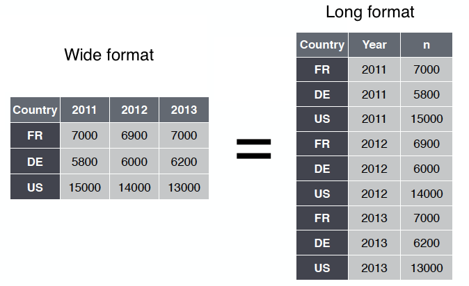
In Module 4, we will see how we can convert a long format to a wide one and vice versa using R.
Additional Resources and Further Reading
Data Wrangling with R by Boehmke (2016) is a comprehensive source for all data types and structures in R. This book is also one the recommended texts in our course. It is available through RMIT Library.
Base R cheatsheet on https://github.com/rstudio/cheatsheets/blob/main/base-r.pdf is useful for remembering commonly used functions and arguments for data types and structures in R.