Summary

Data transformation is perhaps the most important step in the data preprocessing for the development and deployment of statistical analysis and machine learning models. In almost all statistical and machine learning analyses, it is necessary to perform some data transformations (i.e., data transformation, scaling, centering, standardisation and normalisation) on the raw (but tidy and clean!) data before it can be used for modelling.

In this module, first we will focus on the most common and useful data transformations that can be easily implemented in R. The number of possible data transformations is indeed large, and the selection of proper and useful transformations would depend on the context of the data and the type of the statistical analysis. Therefore, specific types of analyses may require specific types of transformations. As you move forward in your master’s program, you will learn the details of these specific transformations used in different data analysis subjects (i.e., Introduction to Statistics, Machine Learning, Analysis of Categorical Data, Time Series Analysis, Forecasting and Applied Bayesian Analysis courses, etc.). Our aim in this course is not to give technical details of these transformations, but you may refer to the “Additional Resources and Further Reading” section to find out more on the topic.

We will also cover brief information on Data Reduction methods and learn when they are used. Please note that we won’t cover the technical details of these methods nor their implementation in R, but you may refer to the “Optional Reading” and “Additional Resources and Further Reading” sections to find out more on the topic. The “Optional Reading” and “Additional Resources and Further Reading” sections won’t be included in the assessments.

Learning Objectives

The learning objectives of this module are as follows:

• Apply well-known transformations.
• Apply normalization and standardization.
• Learn commonly used approaches for data discretisation.
• Gain brief information on different variable selection, ranking and feature extraction techniques for data reduction.

Data Transformation via Mathematical Operations

Often, mathematical operations are applied to the data to achieve normality and/or variance homogeneity. Such transformations through mathematical operations like logarithmic (i.e., ln and log), square root, power transformations etc. can easily be done in R using arithmetic functions.

The most useful transformations in introductory data analysis are the logarithm (base 10 and base e) reciprocal, cube root, square root, and square.

The Log transformation (base 10 - log10 or base e - loge) compresses high values and spreads low values by expressing the values as orders of magnitude. This transformation is commonly used for reducing right skewness. It cannot be applied to zero or negative values directly. In order to apply the log transformation to a zero or negative value, we can add a non-negative constant to all observations and then take the logarithm.

Let’s have a look at the hypothetical data on the salaries data ( salary.csv ).

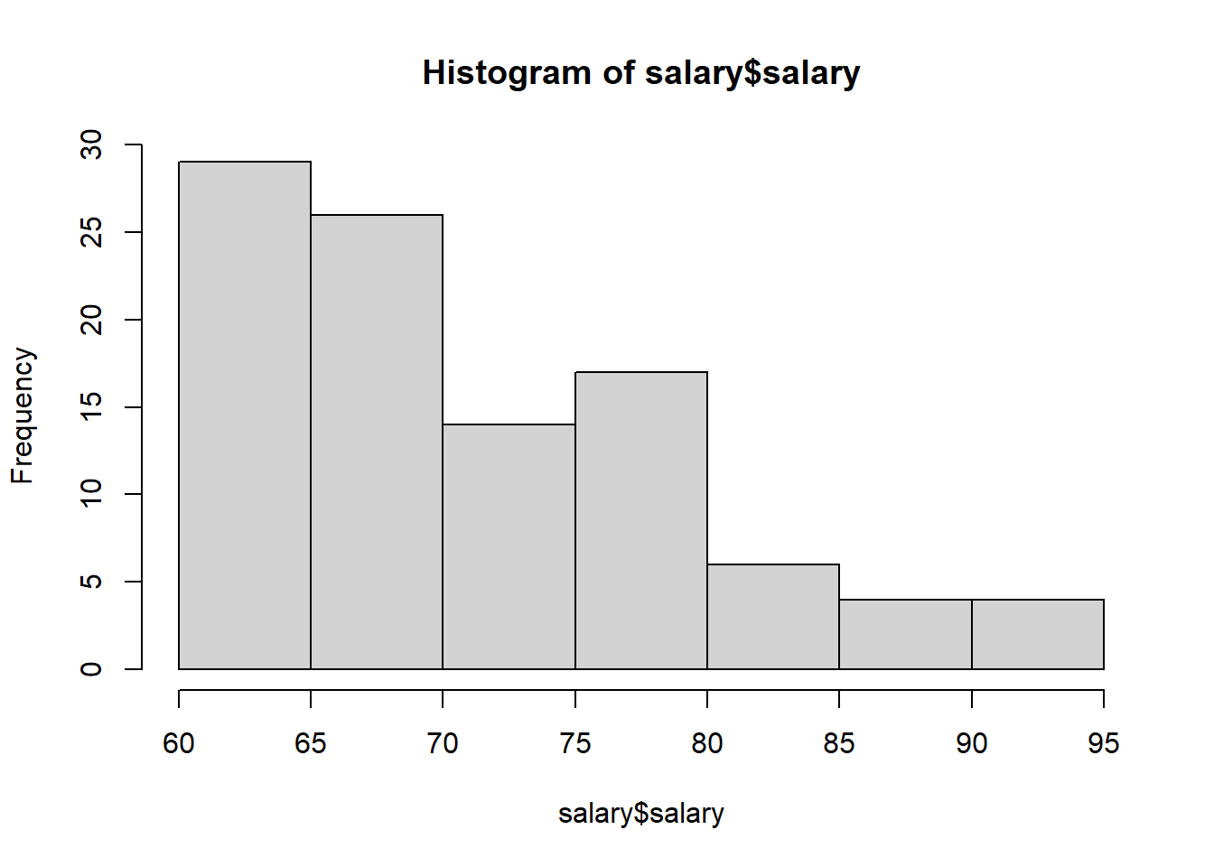
From the histogram, we observe that salaries have a right-skewed distribution. By applying a logarithmic transformation, the salary distribution would be more symmetrical.

We can apply the logarithmic transformation (base 10) using the log10() function in R as follows:

log_salary <- log10(salary$salary)
hist(log_salary)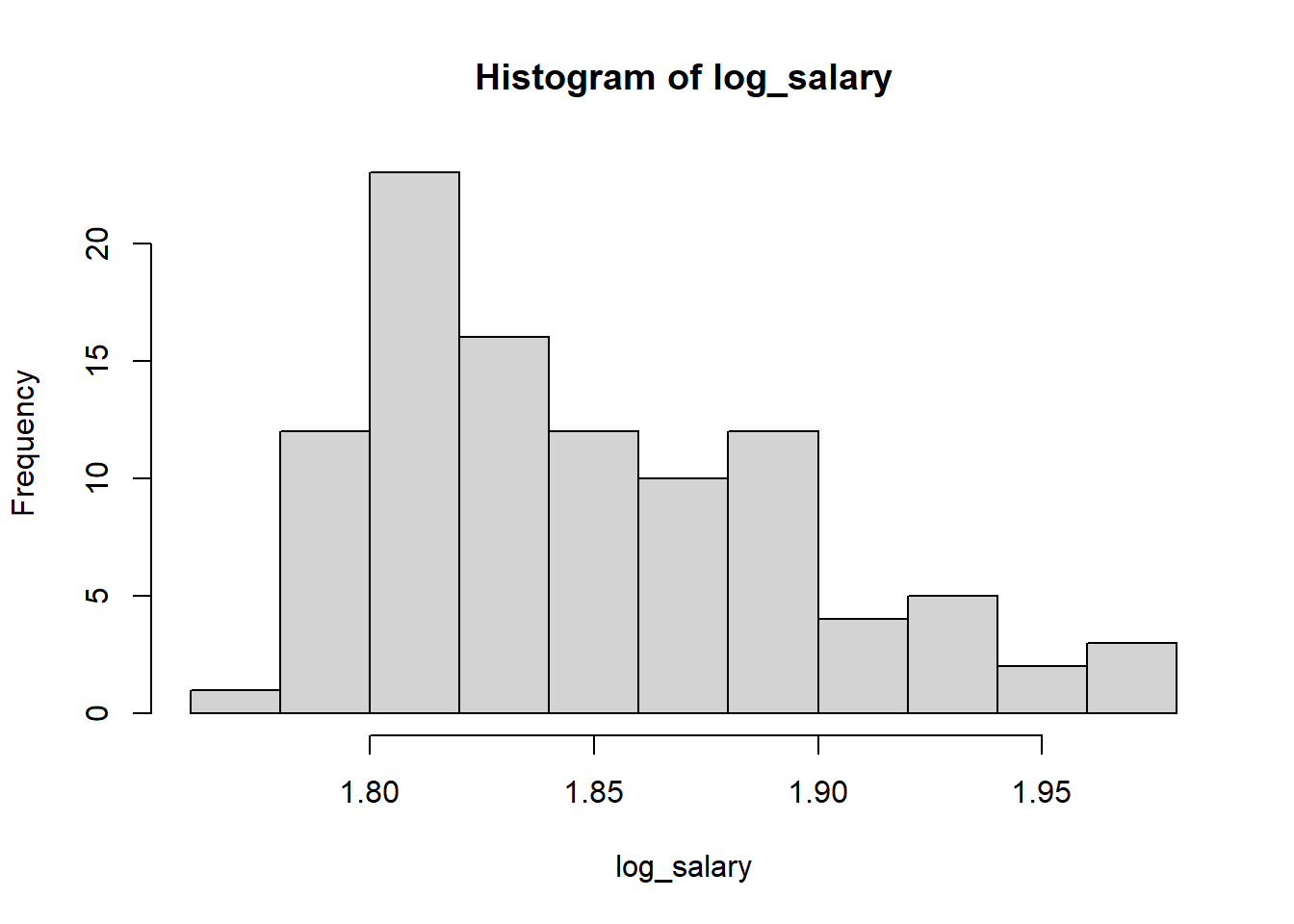

Another logarithmic transformation is the natural logarithm (often called ln or loge). This transformation can be easily done using the log() function in R.

For the salaries data, we can also apply the ln transformation as follows:

ln_salary <- log(salary$salary)
hist(ln_salary)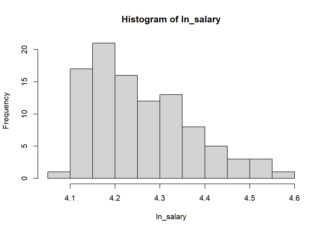

As seen from the histograms, the log10 transformation worked slightly better than the ln transformation for this example. 

Usually, analysts apply different transformations on the same data and then select the one that works well or is useful.

Another transformation is the square root transformation. It is also used for reducing right skewness and has the advantage that it can be applied to zero values. In R, the function sqrt() will apply the square root transformation. Let’s apply the square root transformation and see the effect of this transformation on the salary distribution:

sqrt_salary <- sqrt(salary$salary)
hist(sqrt_salary)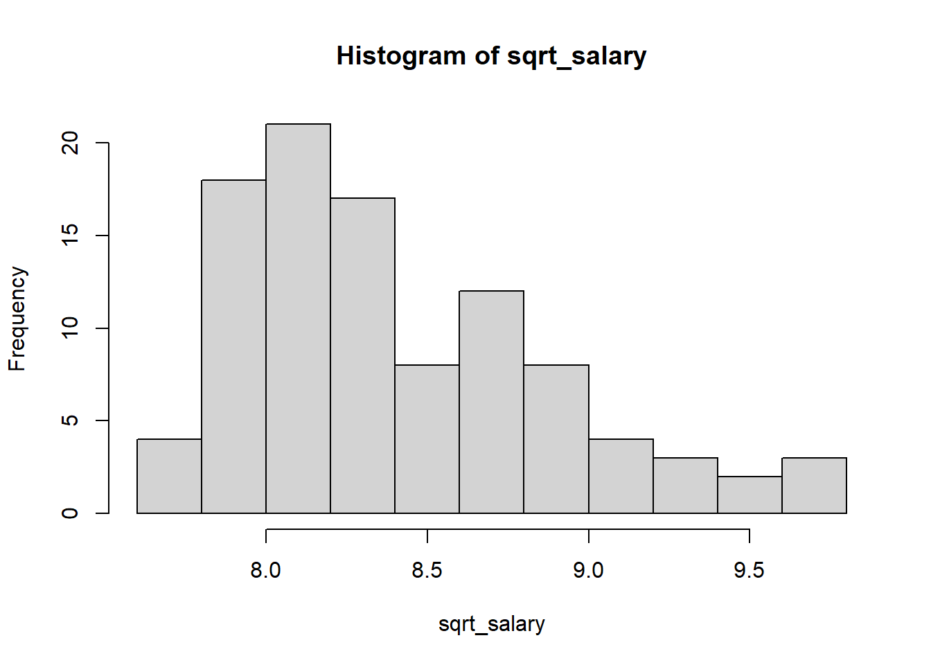

The square root transformation has reduced the skewness in the salary distribution just a bit, however it didn’t completely improve the symmetry of the salary distribution.

The square transformation has a moderate effect on distribution shape and it can be used to reduce left skewness. It spreads out the high values relative to the smaller values. In R, the mathematical operation x^2 would apply the square transformation.

To illustrate the square transformation, let’s read in left_skewed1.csv and have a look at the shape of the distribution using histogram:

x1<- read.csv("data/left_skewed1.csv")

# dropping the first column

x1<-x1[,-1] 
hist(x1)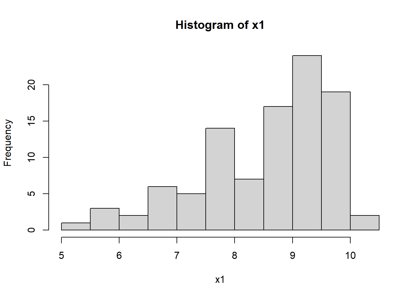

This distribution is left skewed, we can try and see the effect of square transformation on the distribution using the following:

xsquare1 <- x1^2
hist(xsquare1)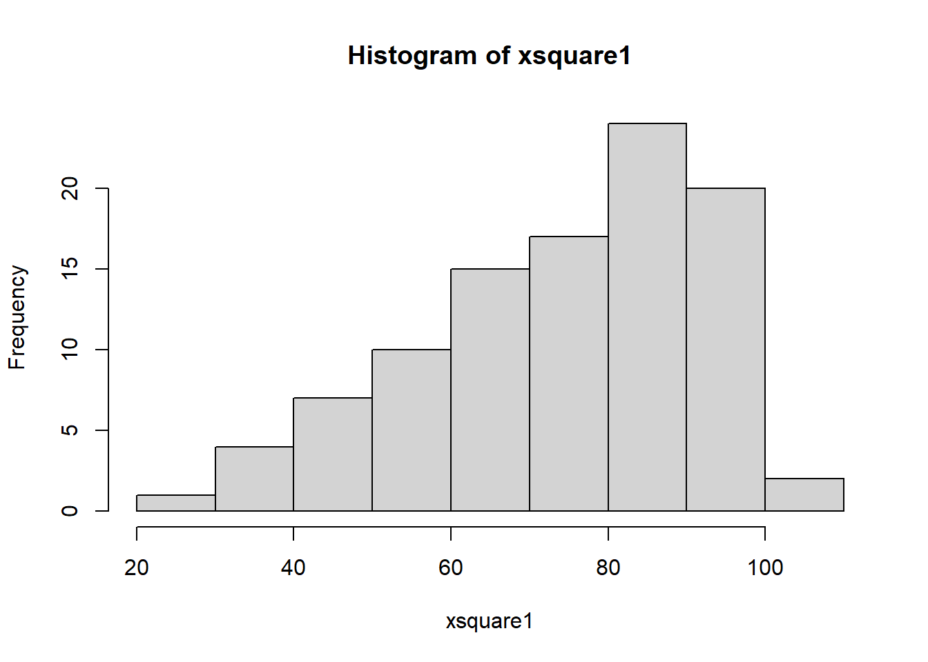

As seen above, the square transformation was not helpful at all to get a symmetrical distribution for this data set. Now, let’s look at another example data left_skewed2.csv having less skewed distribution:

x2<- read.csv("data/left_skewed2.csv")
x2<-x2[,-1] 
hist(x2)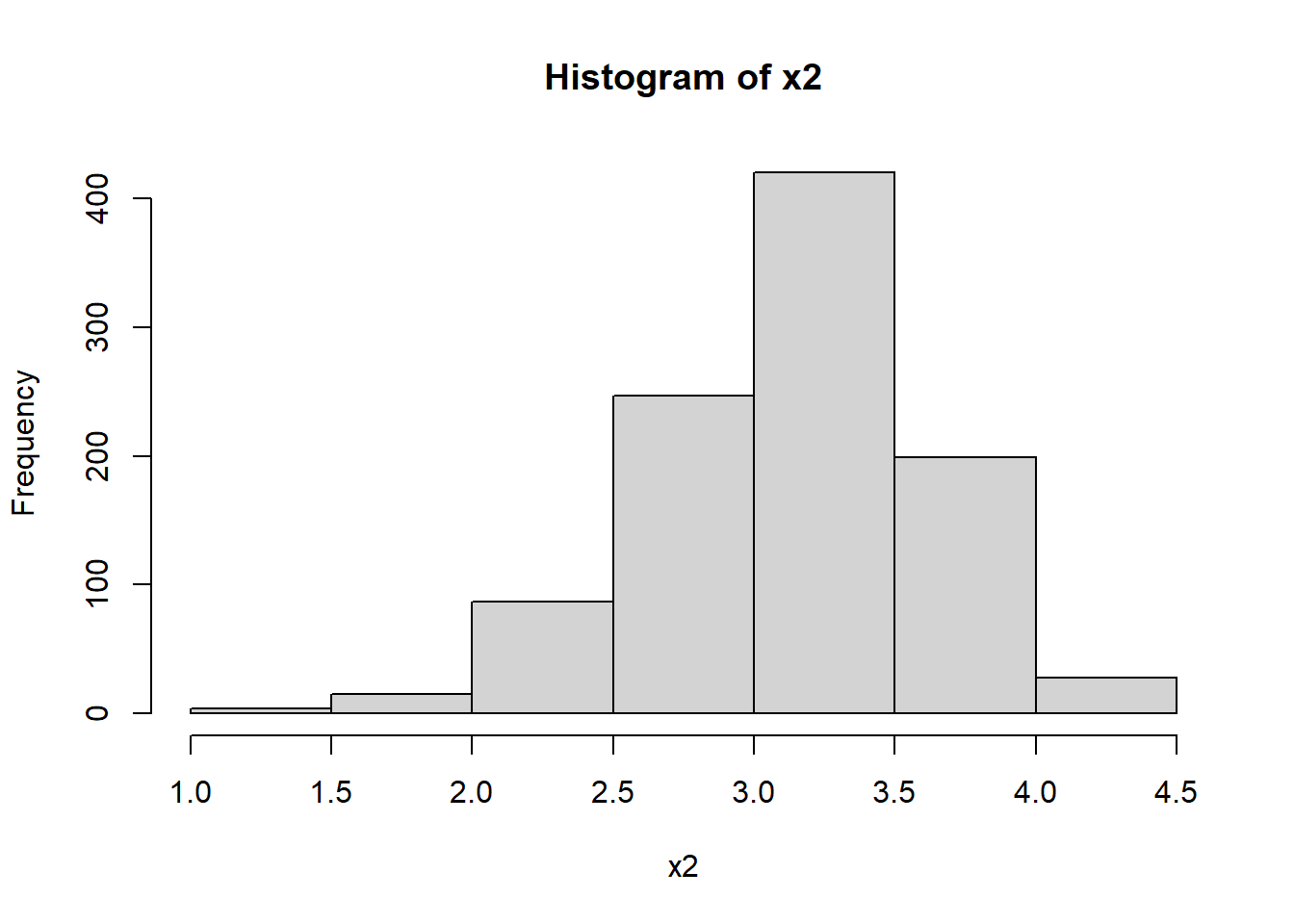

Let’s apply square transformation to x2 and see the effect:

x2square <- x2^2
hist(x2square)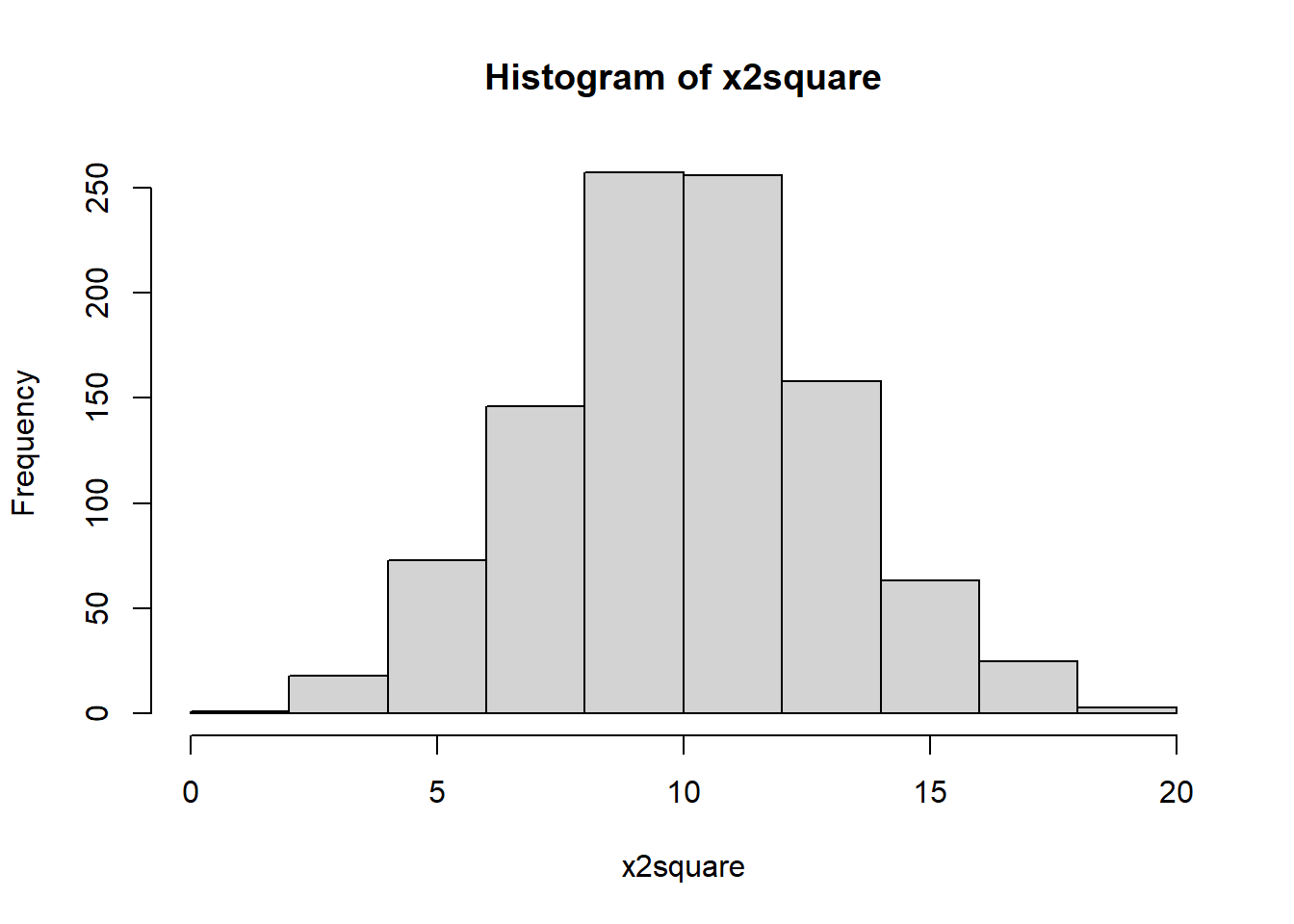

As seen in the last histogram, square transformation was able to transform the shape of the distribution into a more symmetric one when the distribution is mildly left skewed.

The reciprocal transformation is a very strong transformation with a drastic effect on the distribution shape. It will compress large values to smaller values. The mathematical operation 1/xor x^(-1) would apply the reciprocal transformation.

Let’s apply the reciprocal transformation to the x3 variable in the right_skewed1.csv data and see its drastic effect on the shape of the distribution:

x3<- read.csv("data/right_skewed1.csv")
x3<-x3[,-1] 
hist(x3)

x3recip <- 1/x3
hist(x3recip)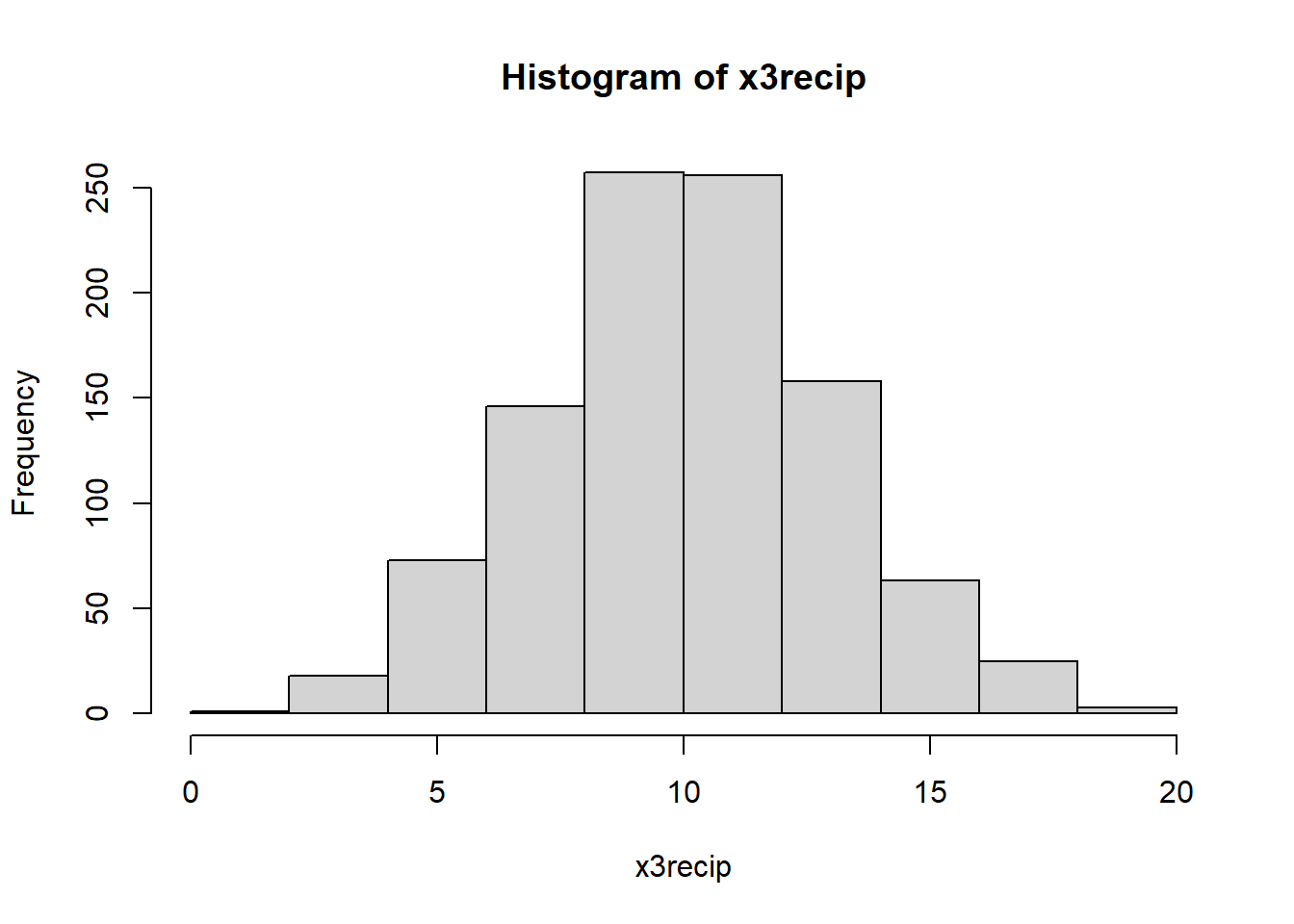

As seen above, reciprocal transformation worked very well in this case.

The main transformations mentioned previously, except for the logarithm, are all powers. Therefore, these transformations are also called as power transformations. Here is the list of power transformations:

Transformation	Power
reciprocal square	-2
reciprocal	-1
(yields one)	0
cube root	1/3
square root	1/2
identity	1
square	2
cube	3
fourth power	4

There are also some recommendations on useful transformations for specific types of distributions. For example:

• To reduce right skewness in the distribution, taking roots or logarithms or reciprocals work well.

• To reduce left skewness, taking squares or cubes or higher powers work well.

Note that these are general recommendations on mathematical transformations and may not work for every data set. Usually, the best approach is to apply different transformations on the same data and select the one that works best.

BoxCox Transformation

Normal distribution assumption is very crucial for many statistical hypothesis tests especially for the parametric hypothesis testing, linear regression, time series analysis, etc. The BoxCox transformation is a type of power transformation to transform non-normal data into a normal distribution. This transformation is named after statisticians George Box and Sir David Cox who collaborated on a 1964 paper and developed the technique (Box and Cox (1964)).

Let y denote the variable at the original scale and y′ the transformed variable. The BoxCox transformation is defined as:

y′={yλ−1λ,if λ≠0log(y),if λ=0

If the data include any negative observations, a shifting parameter λ2 can be included in the BoxCox transformation as given by:

y′={(y+λ2)λ−1λ,if λ≠0log(y+λ2),if λ=0

As seen in the equations, the λ parameter is very important for applying this transformation. Essentially, finding a good λ parameter satisfying the normality assumption is also a hard task and can be done by a search algorithm or the maximum likelihood estimation.

There are many powerful packages that can be used to apply the BoxCox transformation. Among them the caret, MASS, forecast, geoR, EnvStats, and AIS packages are only some of them. In this module, I will introduce the forecast package, as this package has very useful functions to find the best λ parameter for the BoxCox transformation.

#install.packages("forecast")
library(forecast)

To illustrate the BoxCox transformation, let’s revisit the salaries data.

In order to automatically find the best BoxCox transformation parameter λ we can use BoxCox() function using lambda = "auto" argument as follows:

BoxCox_salary<- BoxCox(salary$salary,lambda = "auto")
BoxCox_salary

##   [1] 1.086408 1.084673 1.090454 1.083738 1.084090 1.090965 1.085911 1.089415
##   [9] 1.087011 1.085833 1.089261 1.085384 1.085600 1.083980 1.086385 1.091191
##  [17] 1.086098 1.091735 1.087078 1.085971 1.088653 1.084604 1.088485 1.087204
##  [25] 1.086720 1.090874 1.087691 1.084232 1.088931 1.089373 1.085734 1.085034
##  [33] 1.087939 1.087866 1.087620 1.087019 1.086376 1.083686 1.085093 1.085493
##  [41] 1.087047 1.084546 1.089416 1.092310 1.089200 1.088873 1.085611 1.085940
##  [49] 1.087435 1.083816 1.084803 1.083481 1.083569 1.089794 1.084648 1.090311
##  [57] 1.090420 1.086526 1.084058 1.084592 1.085489 1.086120 1.085241 1.088454
##  [65] 1.088669 1.085080 1.085846 1.083631 1.088054 1.091976 1.086063 1.092688
##  [73] 1.088402 1.087114 1.087016 1.088483 1.084977 1.089249 1.084394 1.084147
##  [81] 1.083339 1.085518 1.085441 1.086812 1.084618 1.085233 1.088769 1.085779
##  [89] 1.085202 1.088973 1.088352 1.086349 1.084721 1.086733 1.089765 1.086601
##  [97] 1.092361 1.090366 1.084704 1.088486
## attr(,"lambda")
## [1] -0.8999268

This function returns the transformed data values. From this output the optimum λ value is found as -0.9999242. We can also see the distribution of transformed values using histogram.

hist(BoxCox_salary)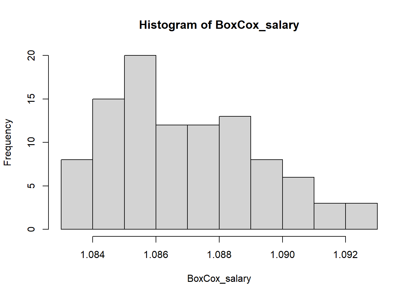

Let’s apply the BoxCox transformation to another data set:

x3<- read.csv("data/right_skewed1.csv")
x3<-x3[,-1] 
hist(x3)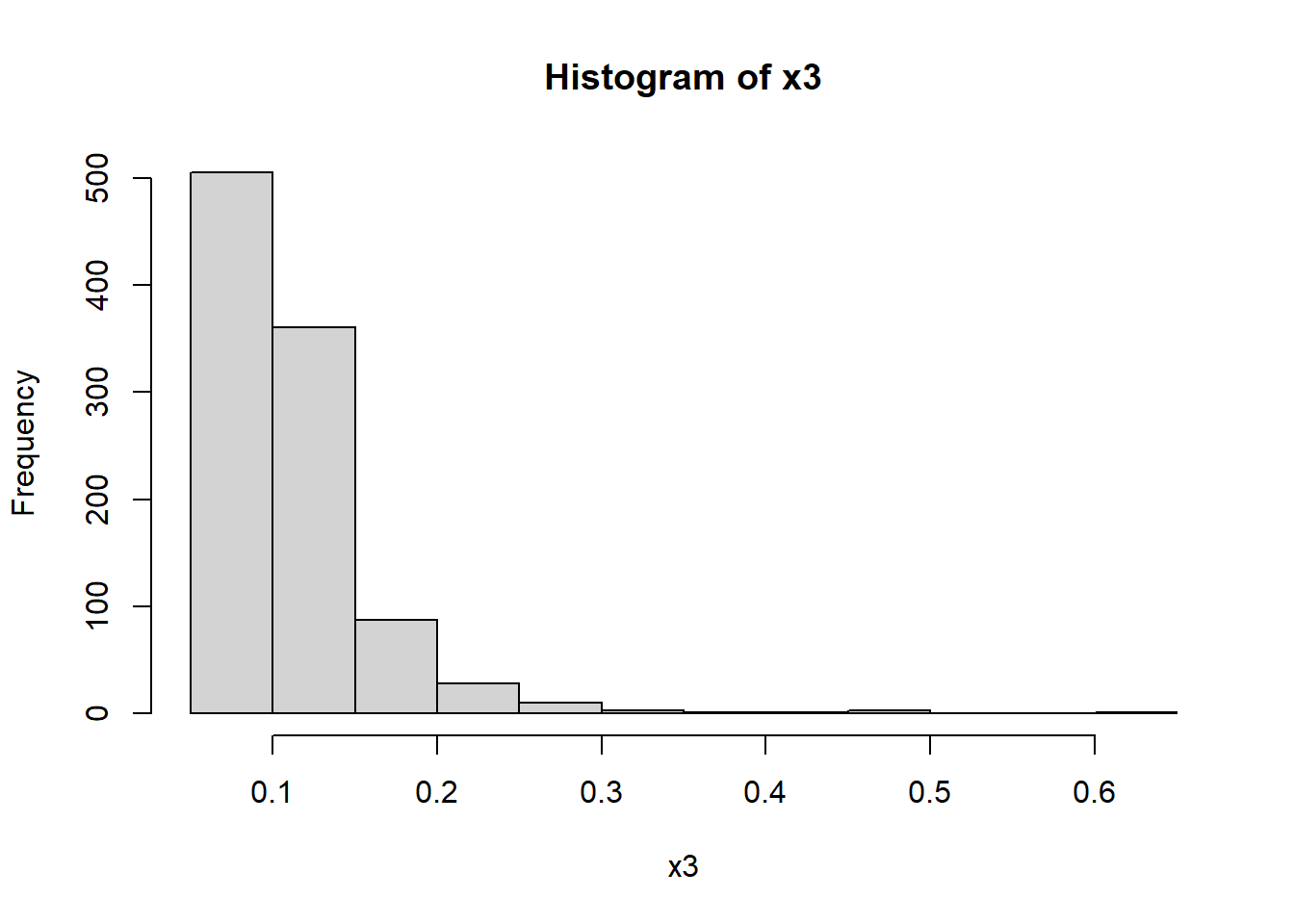

BoxCox_x3<- BoxCox(x3,lambda = "auto")
hist(BoxCox_x3)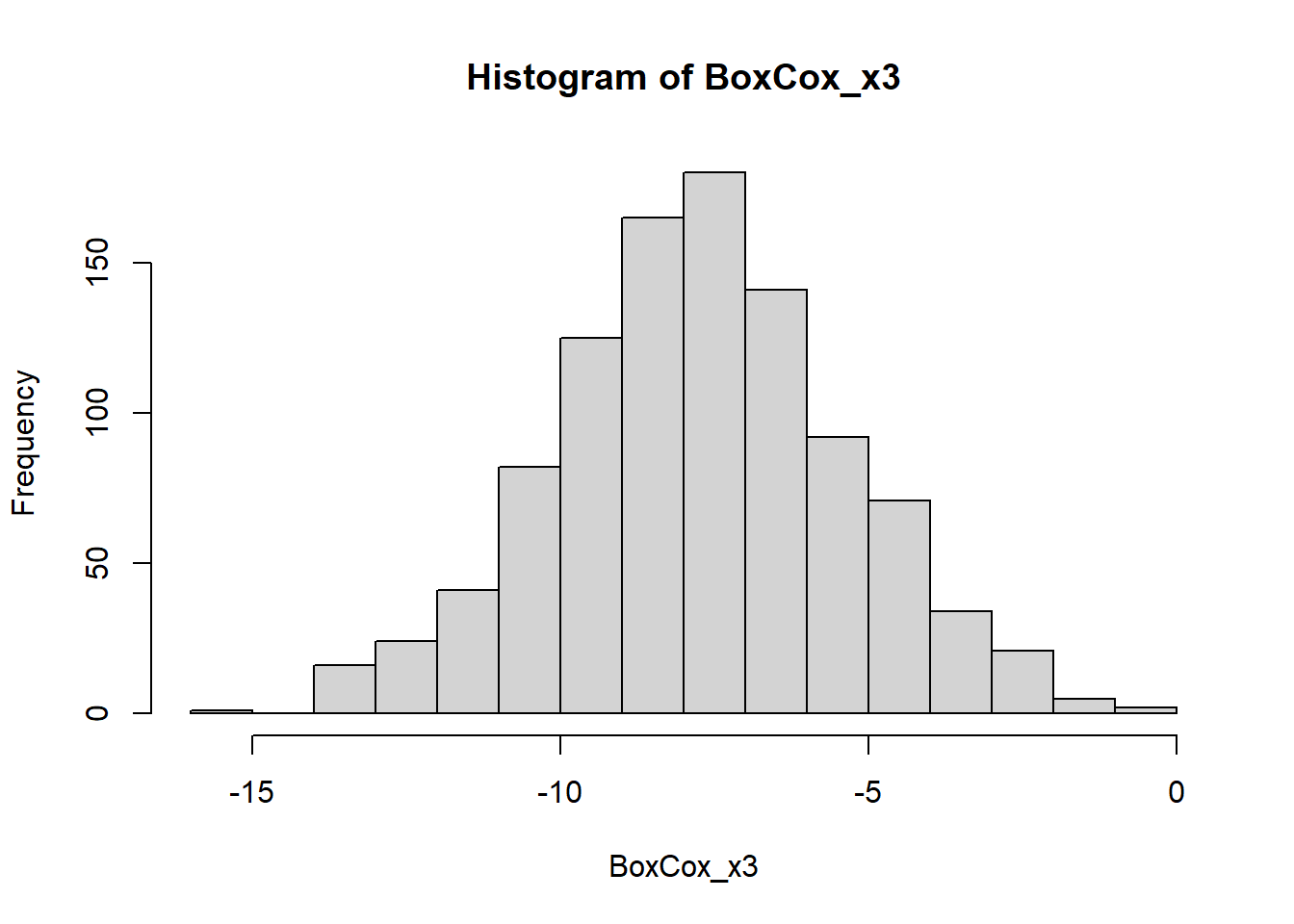

As you can see from the example, the BoxCox transformation is very successful in transforming skewed distributions into a symmetric distribution.

Centering and scaling

Centering (a.k.a. mean-centering) involves the subtraction of the variable average from the data.

Let y denote the variable at the original scale and the ˉy is the average. The centered variable y′ is defined as:

y′=y−ˉy

If we have more than one variable to center, we can calculate the average value of each variable and then subtract it from the data. This implies that each column will be transformed in such a way that the resulting variable will have a zero mean.

We can use simple user-defined functions or built-in functions available in R to center variables. One of the functions to apply mean-centering is the scale() function under Base R. The scale() function has the following arguments:

x: a numeric object

center: if TRUE, the objects’ column means are subtracted from the values in those columns (ignoring NAs); if FALSE, centering is not performed.

scale: if TRUE, the centered column values are divided by the column’s standard deviation (when center is also TRUE) or divided by the root-mean-square (when center is FALSE). If scale = FALSE, scaling is not performed. 

To illustrate centering, let’s take this data frame:

df <- data.frame(x1 = c(10, 20, 40, 50, 10),
                 x2 = c(1000, 5000, 3000, 2000, 1500), 
                 x3 = c(0.1, 0.12, 0.11, 0.14, 0.16), 
                 x4 = c(2.5, 4.2, 3.2, 4.5, 3.8) )

To apply mean-centering, the scale function can be used as follows:

center_df <-scale(df, center = TRUE, scale = FALSE)
center_df

##       x1    x2     x3    x4
## [1,] -16 -1500 -0.026 -1.14
## [2,]  -6  2500 -0.006  0.56
## [3,]  14   500 -0.016 -0.44
## [4,]  24  -500  0.014  0.86
## [5,] -16 -1000  0.034  0.16
## attr(,"scaled:center")
##       x1       x2       x3       x4 
##   26.000 2500.000    0.126    3.640

In the output, the new centered values for each column are given along with the column (variables’) averages.

Scaling involves the division of the values to its standard deviation (or root-mean-square value).

Let y denote the variable at the original scale and the SDy is the standard deviation. The scaled variable y′ is defined as:

y′=ySDy

In order to apply just scaling (without centering) to the data frame we can use center = FALSE and scale = TRUE arguments as follows:

scale_df1 <- scale(df, center = FALSE, scale = TRUE)
scale_df1

##           x1        x2        x3        x4
## [1,] 0.29173 0.3113996 0.6997114 0.6027159
## [2,] 0.58346 1.5569979 0.8396537 1.0125628
## [3,] 1.16692 0.9341987 0.7696826 0.7714764
## [4,] 1.45865 0.6227992 0.9795960 1.0848887
## [5,] 0.29173 0.4670994 1.1195383 0.9161282
## attr(,"scaled:scale")
##           x1           x2           x3           x4 
##   34.2782730 3211.3081447    0.1429161    4.1478910

Note that, when we scale values without centering, the scale() function divides the values to the root-mean-square value instead of standard deviation. Therefore, in this output the new scaled variables are scaled with the column root-mean-square values.

If we want to scale by the standard deviations without centering, we can use the following:

scale_df2 <- scale(df, center = FALSE, scale = apply(df, 2, sd, na.rm = TRUE))
scale_df2

##             x1        x2       x3       x4
## [1,] 0.5504819 0.6324555 4.152274 3.117701
## [2,] 1.1009638 3.1622777 4.982729 5.237738
## [3,] 2.2019275 1.8973666 4.567501 3.990658
## [4,] 2.7524094 1.2649111 5.813184 5.611863
## [5,] 0.5504819 0.9486833 6.643638 4.738906
## attr(,"scaled:scale")
##           x1           x2           x3           x4 
## 1.816590e+01 1.581139e+03 2.408319e-02 8.018728e-01

The output above now reports the scaled values (by standard deviation) along with the column standard deviations.

Usually, scaling is not used alone, instead, it is used together with mean-centering and then it is called as the z-score standardisation.

z score standardisation

Note that in Module 6, we have already seen the z-scores and we used them to detect the outliers. In the z-score transformation, the mean of observations is first subtracted from each individual data point, then divided by the standard deviation of all points. The resulting transformed data values would have a zero mean and one standard deviation. The z-score transformation can be applied using the following equation:

z=y−ˉySDy

In the equation below, y denotes the values of observations, ˉy and SDy are the sample mean and standard deviation, respectively.

The z-score transformation can also be applied using the scale() with the center = TRUE, scale = TRUE arguments.

z_df <- scale(df, center = TRUE, scale = TRUE)
z_df

##              x1         x2         x3         x4
## [1,] -0.8807710 -0.9486833 -1.0795912 -1.4216719
## [2,] -0.3302891  1.5811388 -0.2491364  0.6983651
## [3,]  0.7706746  0.3162278 -0.6643638 -0.5487155
## [4,]  1.3211565 -0.3162278  0.5813184  1.0724893
## [5,] -0.8807710 -0.6324555  1.4117732  0.1995329
## attr(,"scaled:center")
##       x1       x2       x3       x4 
##   26.000 2500.000    0.126    3.640 
## attr(,"scaled:scale")
##           x1           x2           x3           x4 
## 1.816590e+01 1.581139e+03 2.408319e-02 8.018728e-01

Note that we can also use other functions (i.e., scores()) from other packages to get the same result.

Min- Max Normalisation (a.k.a. range or (0-1) normalization)

An alternative approach to z-score standardization is the Min-Max normalization technique which specifies the following formula to be applied to each value of features to be normalized.

y′=y−yminymax−ymin

In this approach, the data is scaled to a fixed range - usually 0 to 1. Therefore, sometimes this method is called (0-1) normalization. In contrast to z-score standardization this normalization can suppress the effect of outliers.

In R, the min-max normalization can be applied in many ways and the simplest way would be writing a function like the following:

minmaxnormalise <- function(x){(x- min(x)) /(max(x)-min(x))}

Then, using lapply() one can apply this function to a data frame.

lapply(df, minmaxnormalise)

## $x1
## [1] 0.00 0.25 0.75 1.00 0.00
## 
## $x2
## [1] 0.000 1.000 0.500 0.250 0.125
## 
## $x3
## [1] 0.0000000 0.3333333 0.1666667 0.6666667 1.0000000
## 
## $x4
## [1] 0.00 0.85 0.35 1.00 0.65

If you would like to store the normalized values as a data frame you may also use as.data.frame() function:

as.data.frame(lapply(df, minmaxnormalise))

##     x1    x2        x3   x4
## 1 0.00 0.000 0.0000000 0.00
## 2 0.25 1.000 0.3333333 0.85
## 3 0.75 0.500 0.1666667 0.35
## 4 1.00 0.250 0.6666667 1.00
## 5 0.00 0.125 1.0000000 0.65

Equal width (distance) binning

In equal-width binning, the variable is divided into n intervals of equal size. If ymax and ymin are the maximum and the minimum values in the variable, the width of the intervals will be:

w=ymax−yminn

Thus, we need to define the number of intervals n prior to binning. However, this is not an easy task for the analysts and constitutes one of the disadvantages of this method.

In R, we can use the discretize() function under the infotheo package to apply an equal-width binning.

#install.packages("infotheo")
library(infotheo)

To illustrate binning using equal width, let’s revisit the subset of the iris data set.

# load iris data and subset using versicolor flowers, with the first three variables

iris <- read.csv("data/iris.csv")
versicolor <- iris %>% filter( Species == "versicolor" ) %>% dplyr::select(Sepal.Length)
head(versicolor)

##   Sepal.Length
## 1          7.0
## 2          6.4
## 3          6.9
## 4          5.5
## 5          6.5
## 6          5.7

Let’s apply equal-width binning to the Sepal.Length variable.

ew_binned<-discretize(versicolor, disc = "equalwidth")
versicolor %>% bind_cols(ew_binned) %>% head(15)

## New names:
## • `Sepal.Length` -> `Sepal.Length...1`
## • `Sepal.Length` -> `Sepal.Length...2`

##    Sepal.Length...1 Sepal.Length...2
## 1               7.0                3
## 2               6.4                3
## 3               6.9                3
## 4               5.5                1
## 5               6.5                3
## 6               5.7                2
## 7               6.3                3
## 8               4.9                1
## 9               6.6                3
## 10              5.2                1
## 11              5.0                1
## 12              5.9                2
## 13              6.0                2
## 14              6.1                2
## 15              5.6                1

Equal depth (frequency) binning

In equal-depth binning method, the variable is divided into n intervals, each containing approximately the same number of observations (frequencies).

In R, we can use the discretize() function with disc = "equalfreq" argument to apply this method.

To apply equal-depth binning to the Sepal.Length variable.

ed_binned<-discretize(versicolor, disc = "equalfreq")
versicolor %>% bind_cols(ed_binned) %>% head(15)

## New names:
## • `Sepal.Length` -> `Sepal.Length...1`
## • `Sepal.Length` -> `Sepal.Length...2`

##    Sepal.Length...1 Sepal.Length...2
## 1               7.0                3
## 2               6.4                3
## 3               6.9                3
## 4               5.5                1
## 5               6.5                3
## 6               5.7                1
## 7               6.3                3
## 8               4.9                1
## 9               6.6                3
## 10              5.2                1
## 11              5.0                1
## 12              5.9                2
## 13              6.0                2
## 14              6.1                2
## 15              5.6                1

Feature filtering

In feature filtering, redundant features are filtered out and the ones that are most useful or most relevant for the problem are selected. Feature filtering methods include removing features with zero and near zero-variance and removing highly correlated variables (i.e., greater than 0.8).

Feature ranking

This method includes ranking features according to an importance criterion and selecting those which are above a defined threshold. This technique is also called feature ranking. In this technique features are ranked according to a statistical criterion (i.e., chi-square test, correlation test, entropy-based tests, random forest, etc.) and either selected to be kept or removed from the data set.

Principal Component Analysis (PCA)

This method is an unsupervised algorithm that creates linear combinations of the original features. The new extracted features are orthogonal, which means that they are uncorrelated. The extracted components are ranked in order of their “explained variance”. For example, the first principal component (PC1) explains the most variance in the data, PC2 explains the second-most variance, and so on. Then you can decide to keep only as many principal components as needed to reach a cumulative explained variance of 90%. Note that the advantage of this technique is fast and simple to implement and works well in practice. However, the new principal components are not interpretable, because they are linear combinations of original features. 

PCA is used to analyse each variable’s (i.e. component’s) relation to the variance. It gives the variance for each component, and then allows the user to decide as to which components should be included in the analysis to prevent overfitting the model. The first component outputted has the highest variance, the second is lower and so on.

Principal component analysis is also a broad topic in Multivariate statistical analysis. For more information on PCA please refer to the references given under “Additional Resources and Further Reading” section.

A quick look to the mlr package

There are many powerful packages that can be used in dimension reduction. Most of them are essentially used for machine learning tasks and they also provide specific functions for feature selection and extraction.

The mlr package is an all-in-one package that offers most of the data preprocessing tasks (i.e. missing values imputation, normalising, centering, standardising, transforming, feature extraction and selection) required in machine learning analysis.

To start with the main features of the mlr package, I will use a simple example of regression analysis on the iris data set. First, we need to install and load the mlr package:

#install.packages("mlr")
library(mlr)

The entire structure of mlr package relies on the following steps:

1. Create a task -> 2. Create a learner -> 3. Fit a model -> 4. Make predictions -> 5. Evaluate the learner
   

1. Create a task

Creating a task means specifying the type of analysis and providing the data and response variable. The makeClassifTask() function will define the task as a classification, similarly makeRegrTask() will specify the task as a regression analysis. Note that the full list of available tasks for this step can be found in the mlr package tutorial (https://mlr.mlr-org.com/articles/tutorial/task.html)

Let’s illustrate this step using the BostonHousing data set. Assume that we would like to predict the medv using other variables. Then we can specify the task and the data as follows:

data(BostonHousing)

# 1) Define the task
# Specify the type of analysis (e.g. regression) and provide data and response variable

BostonHousing.task = makeRegrTask(data = BostonHousing, target = "medv")

2. Create a learner

Creating a learner means choosing a specific algorithm (learner) which learns from task (or data). With makeLearner() function we can easily specify the learner.

Let’s specify the learner algorithm as the generalized linear model (a.k.a classical regression) using:

# 2) Define the learner
# Choose a specific algorithm (e.g. generalized linear model - classical regression)

lrn = makeLearner("regr.glm")

Note that the full list for available learners can be found in (https://mlr.mlr-org.com/)

3. Fit the model

Fitting the model means use a random subset of data (i.e. training set) to develop/fit a model. The train() function will define the model in the train set.

First, we need to divide the data set into train and test sets. We can use sample() from Base R and setdiff() from dplyr package:

# Divide the data set into train and test sets

n = nrow(BostonHousing)
train.set = sample(n, size = 2/3*n)
test.set = setdiff(1:n, train.set)

# 3) Fit the model
# Train the learner on the task using a random subset of the data as training set

model = mlr::train(lrn, BostonHousing.task, subset = train.set)

4. Make predictions

Making predictions means applying the model in the test set and predicting the response for new observations. The predict() function will predict the response variable for the new observations.

# 4) Make predictions
# Predict values of the response variable for new observations by the trained model using the other part of the data as test set

pred = predict(model, task = BostonHousing.task, subset = test.set)

5. Evaluate the learner

This step includes the calculation of performance metrics (e.g. mean misclassification error and accuracy) for learners. The performance() function will easily define the evaluation metrics.

# 5) Evaluate the learner
# Calculate the mean squared error and mean absolute error

performance(pred, measures = list(mse, mae))

##       mse       mae 
## 16.076245  3.130626

So far, the main workflow of mlr package is introduced in a general sense. In the next sections we will see the details of how to use these functions for feature selection and feature extraction.

Example on Feature Filtering

To illustrate feature filtering, we will continue with the BostonHousing.task (given above). In the BostonHousing data frame, we have 14 features (one of them medv is defined as response/target variable).

BostonHousing.task

## Supervised task: BostonHousing
## Type: regr
## Target: medv
## Observations: 506
## Features:
##    numerics     factors     ordered functionals 
##          12           1           0           0 
## Missings: FALSE
## Has weights: FALSE
## Has blocking: FALSE
## Has coordinates: FALSE

# Print the feature names in the task

getTaskFeatureNames(BostonHousing.task)

##  [1] "crim"    "zn"      "indus"   "chas"    "nox"     "rm"      "age"    
##  [8] "dis"     "rad"     "tax"     "ptratio" "b"       "lstat"

To drop specific features, let’s say age, we can use dropFeatures(task, features) function.

# Drop the age and write it into the BostonHousing.task1

BostonHousing.task1 <-dropFeatures(BostonHousing.task, features = "age")
BostonHousing.task1

## Supervised task: BostonHousing
## Type: regr
## Target: medv
## Observations: 506
## Features:
##    numerics     factors     ordered functionals 
##          11           1           0           0 
## Missings: FALSE
## Has weights: FALSE
## Has blocking: FALSE
## Has coordinates: FALSE

# Print the feature names

getTaskFeatureNames(BostonHousing.task1)

##  [1] "crim"    "zn"      "indus"   "chas"    "nox"     "rm"      "dis"    
##  [8] "rad"     "tax"     "ptratio" "b"       "lstat"

Example on Principle Component Analysis

In R, we can apply principal component analysis using many different packages (like prcomp(), caret, etc). Essentially, the mlr package that we used for feature ranking and selection, uses caret package and functions behind to apply feature extraction.

I will use the caret package to demonstrate the data extraction as it has a straightforward usage. Please note that any caret functions can also be converted into the mlr functions. For more information on this conversion, you can refer to the mlr package manual.

In the caret package you simply apply PCA analysis using preProcess() function as follows:

library(caret)

I will use another example called sonar signals data task which is already available under the mlbench package to further illustrate feature extraction.

# to load the sonar data

library(mlbench) 

Note that this data has 208 observations and 60 features. Let’s look at the header of the sonar data:

data(Sonar)
head(Sonar)

##       V1     V2     V3     V4     V5     V6     V7     V8     V9    V10    V11
## 1 0.0200 0.0371 0.0428 0.0207 0.0954 0.0986 0.1539 0.1601 0.3109 0.2111 0.1609
## 2 0.0453 0.0523 0.0843 0.0689 0.1183 0.2583 0.2156 0.3481 0.3337 0.2872 0.4918
## 3 0.0262 0.0582 0.1099 0.1083 0.0974 0.2280 0.2431 0.3771 0.5598 0.6194 0.6333
## 4 0.0100 0.0171 0.0623 0.0205 0.0205 0.0368 0.1098 0.1276 0.0598 0.1264 0.0881
## 5 0.0762 0.0666 0.0481 0.0394 0.0590 0.0649 0.1209 0.2467 0.3564 0.4459 0.4152
## 6 0.0286 0.0453 0.0277 0.0174 0.0384 0.0990 0.1201 0.1833 0.2105 0.3039 0.2988
##      V12    V13    V14    V15    V16    V17    V18    V19    V20    V21    V22
## 1 0.1582 0.2238 0.0645 0.0660 0.2273 0.3100 0.2999 0.5078 0.4797 0.5783 0.5071
## 2 0.6552 0.6919 0.7797 0.7464 0.9444 1.0000 0.8874 0.8024 0.7818 0.5212 0.4052
## 3 0.7060 0.5544 0.5320 0.6479 0.6931 0.6759 0.7551 0.8929 0.8619 0.7974 0.6737
## 4 0.1992 0.0184 0.2261 0.1729 0.2131 0.0693 0.2281 0.4060 0.3973 0.2741 0.3690
## 5 0.3952 0.4256 0.4135 0.4528 0.5326 0.7306 0.6193 0.2032 0.4636 0.4148 0.4292
## 6 0.4250 0.6343 0.8198 1.0000 0.9988 0.9508 0.9025 0.7234 0.5122 0.2074 0.3985
##      V23    V24    V25    V26    V27    V28    V29    V30    V31    V32    V33
## 1 0.4328 0.5550 0.6711 0.6415 0.7104 0.8080 0.6791 0.3857 0.1307 0.2604 0.5121
## 2 0.3957 0.3914 0.3250 0.3200 0.3271 0.2767 0.4423 0.2028 0.3788 0.2947 0.1984
## 3 0.4293 0.3648 0.5331 0.2413 0.5070 0.8533 0.6036 0.8514 0.8512 0.5045 0.1862
## 4 0.5556 0.4846 0.3140 0.5334 0.5256 0.2520 0.2090 0.3559 0.6260 0.7340 0.6120
## 5 0.5730 0.5399 0.3161 0.2285 0.6995 1.0000 0.7262 0.4724 0.5103 0.5459 0.2881
## 6 0.5890 0.2872 0.2043 0.5782 0.5389 0.3750 0.3411 0.5067 0.5580 0.4778 0.3299
##      V34    V35    V36    V37    V38    V39    V40    V41    V42    V43    V44
## 1 0.7547 0.8537 0.8507 0.6692 0.6097 0.4943 0.2744 0.0510 0.2834 0.2825 0.4256
## 2 0.2341 0.1306 0.4182 0.3835 0.1057 0.1840 0.1970 0.1674 0.0583 0.1401 0.1628
## 3 0.2709 0.4232 0.3043 0.6116 0.6756 0.5375 0.4719 0.4647 0.2587 0.2129 0.2222
## 4 0.3497 0.3953 0.3012 0.5408 0.8814 0.9857 0.9167 0.6121 0.5006 0.3210 0.3202
## 5 0.0981 0.1951 0.4181 0.4604 0.3217 0.2828 0.2430 0.1979 0.2444 0.1847 0.0841
## 6 0.2198 0.1407 0.2856 0.3807 0.4158 0.4054 0.3296 0.2707 0.2650 0.0723 0.1238
##      V45    V46    V47    V48    V49    V50    V51    V52    V53    V54    V55
## 1 0.2641 0.1386 0.1051 0.1343 0.0383 0.0324 0.0232 0.0027 0.0065 0.0159 0.0072
## 2 0.0621 0.0203 0.0530 0.0742 0.0409 0.0061 0.0125 0.0084 0.0089 0.0048 0.0094
## 3 0.2111 0.0176 0.1348 0.0744 0.0130 0.0106 0.0033 0.0232 0.0166 0.0095 0.0180
## 4 0.4295 0.3654 0.2655 0.1576 0.0681 0.0294 0.0241 0.0121 0.0036 0.0150 0.0085
## 5 0.0692 0.0528 0.0357 0.0085 0.0230 0.0046 0.0156 0.0031 0.0054 0.0105 0.0110
## 6 0.1192 0.1089 0.0623 0.0494 0.0264 0.0081 0.0104 0.0045 0.0014 0.0038 0.0013
##      V56    V57    V58    V59    V60 Class
## 1 0.0167 0.0180 0.0084 0.0090 0.0032     R
## 2 0.0191 0.0140 0.0049 0.0052 0.0044     R
## 3 0.0244 0.0316 0.0164 0.0095 0.0078     R
## 4 0.0073 0.0050 0.0044 0.0040 0.0117     R
## 5 0.0015 0.0072 0.0048 0.0107 0.0094     R
## 6 0.0089 0.0057 0.0027 0.0051 0.0062     R

In this example, I will apply a PCA analysis and keep only as many principal components as needed to reach a cumulative explained variance of 90% by specifying thresh = 0.90 argument.

pca1 <- preProcess(Sonar, method = "pca", thresh = 0.90)
pca1

## Created from 208 samples and 61 variables
## 
## Pre-processing:
##   - centered (60)
##   - ignored (1)
##   - principal component signal extraction (60)
##   - scaled (60)
## 
## PCA needed 22 components to capture 90 percent of the variance

According to the summary output, the PCA extracted 22 components to reach a cumulative explained variance of 90%. Note that the variables were centered and scaled in default for this analysis. We can inspect the extracted components using pca1$rotation.

head(pca1$rotation)

##           PC1        PC2          PC3         PC4        PC5        PC6
## V1 0.13637827 -0.1223047  0.015992208 -0.01398332 0.13559873 -0.1102138
## V2 0.14605308 -0.1310784  0.016703474 -0.06095574 0.16977542 -0.1432289
## V3 0.11572088 -0.1424144  0.008359428 -0.11166025 0.18842191 -0.2173942
## V4 0.09390192 -0.1544207 -0.023779899 -0.10136333 0.17819174 -0.2512730
## V5 0.05534548 -0.1604564  0.025419982 -0.07332698 0.07256160 -0.2126554
## V6 0.05175506 -0.1458544  0.068286250  0.10835565 0.06708443 -0.1715077
##            PC7         PC8         PC9        PC10         PC11        PC12
## V1  0.06587748 -0.03328692 0.037186619 -0.25134519  0.097850678 -0.24260274
## V2  0.05676022 -0.11883210 0.091322333 -0.23737187  0.121550063 -0.18752348
## V3  0.02440144 -0.21242355 0.021327006 -0.15446882  0.089056158 -0.19831618
## V4  0.01098851 -0.18558617 0.001593686 -0.17478173 -0.008240723 -0.02783503
## V5 -0.10501142 -0.25891923 0.030974131 -0.12111680 -0.077089767  0.22377684
## V6 -0.23261559 -0.14769658 0.175673115  0.04487812 -0.254604172  0.32464660
##            PC13         PC14        PC15        PC16        PC17        PC18
## V1  0.005952877 -0.164560269  0.03655007 -0.17522136  0.25687921 -0.10407706
## V2  0.037133404 -0.009202382  0.16264602 -0.12151447  0.21693382 -0.02226816
## V3 -0.094157030  0.089266763  0.05240022  0.08930538  0.05841650  0.09402403
## V4 -0.179494903  0.088033831 -0.03178224  0.10546228 -0.11760130  0.08075530
## V5 -0.263286223  0.150051748 -0.09714955 -0.13689196 -0.19561809  0.06066290
## V6  0.005002015  0.018717413  0.03693093 -0.21681823 -0.05577494  0.07362170
##            PC19         PC20        PC21        PC22
## V1  0.331965391 -0.034181265 -0.07401342 -0.09951057
## V2  0.042911886  0.042456268 -0.13738490 -0.06477669
## V3 -0.175998680 -0.007611349 -0.05533080 -0.05188087
## V4 -0.089819019  0.092698570  0.20131836  0.07823582
## V5 -0.013490921  0.109094193  0.22218307 -0.01440086
## V6 -0.001379493 -0.075714035 -0.15151985 -0.13217653

As seen in the output, the PCA analysis extracted 22 so-called components. These components are uncorrelated (orthogonal to each other) and they have no specific interpretation. However, the advantage is extracting and using 22 new components instead of 60 (original features in the sonar data) would definitely help us with the “curse of dimensionality” problem.

When we have a prior knowledge on the number of dimensions, we can also set the specific number of PCA components to keep using the pcaComp argument.

pca2 <- preProcess(Sonar, method = "pca", pcaComp = 3)
pca2

## Created from 208 samples and 61 variables
## 
## Pre-processing:
##   - centered (60)
##   - ignored (1)
##   - principal component signal extraction (60)
##   - scaled (60)
## 
## PCA used 3 components as specified

In this example, I applied a PCA analysis with 3 components by specifying pcaComp = 3 argument. We can further inspect the extracted components using pca2$rotation.

pca2$rotation

##              PC1          PC2          PC3
## V1   0.136378273 -0.122304688  0.015992208
## V2   0.146053080 -0.131078408  0.016703474
## V3   0.115720878 -0.142414435  0.008359428
## V4   0.093901919 -0.154420728 -0.023779899
## V5   0.055345485 -0.160456428  0.025419982
## V6   0.051755057 -0.145854449  0.068286250
## V7   0.062775610 -0.140891454  0.074614661
## V8   0.105054791 -0.134863768  0.079735581
## V9   0.098197274 -0.119155949  0.101057756
## V10  0.087921207 -0.124444064  0.114638424
## V11  0.057375857 -0.157682950  0.147757860
## V12  0.030813905 -0.135537002  0.136074294
## V13  0.020969659 -0.184297302  0.128481313
## V14  0.005652117 -0.231772023  0.054958097
## V15 -0.004990611 -0.237948698 -0.011431980
## V16 -0.016056791 -0.238450888 -0.044277247
## V17 -0.051234729 -0.222494179 -0.056807261
## V18 -0.083791662 -0.213388066 -0.080813285
## V19 -0.081184281 -0.216616457 -0.044392022
## V20 -0.062915260 -0.209771922 -0.026074932
## V21 -0.078740257 -0.187687956  0.015968283
## V22 -0.129462677 -0.135829504  0.099660597
## V23 -0.148562415 -0.066017595  0.136056233
## V24 -0.153926815 -0.009777176  0.170925676
## V25 -0.157453398  0.040652190  0.205383077
## V26 -0.146949892  0.082056910  0.226717362
## V27 -0.124882420  0.112139679  0.239775863
## V28 -0.049328849  0.155239754  0.233097760
## V29 -0.010665698  0.184510827  0.179959425
## V30  0.065818390  0.175836616  0.114940670
## V31  0.091115681  0.169186361  0.092560311
## V32  0.111811541  0.157449080  0.043486178
## V33  0.126459063  0.158206935 -0.080488798
## V34  0.143923355  0.124475481 -0.178375368
## V35  0.153260435  0.097467158 -0.214919829
## V36  0.152803748  0.086956751 -0.216069266
## V37  0.149774729  0.062682339 -0.204157446
## V38  0.185056839  0.041297372 -0.172220813
## V39  0.188787349  0.025641186 -0.112743470
## V40  0.179847963  0.036702231 -0.096129734
## V41  0.201924499  0.044193536 -0.027451916
## V42  0.198203989  0.040442163  0.072415268
## V43  0.184618686  0.056311358  0.142594404
## V44  0.170194631  0.054520494  0.163327534
## V45  0.200815274  0.028724431  0.191981350
## V46  0.199261298  0.034322885  0.196152753
## V47  0.177099699  0.029529461  0.226575253
## V48  0.184090972  0.009544262  0.215221572
## V49  0.175503993 -0.012209874  0.207469384
## V50  0.158819355 -0.019105674  0.127570395
## V51  0.145283851 -0.054479908  0.167847245
## V52  0.139679711 -0.068751303  0.106799738
## V53  0.123721695 -0.068411996 -0.006644230
## V54  0.115164579 -0.107073180 -0.023156403
## V55  0.127573257 -0.109155326 -0.032838063
## V56  0.113651055 -0.097333904 -0.032792805
## V57  0.112250706 -0.086072801 -0.045159077
## V58  0.134271001 -0.110317668 -0.017004846
## V59  0.143756315 -0.090282629 -0.072818633
## V60  0.117841717 -0.075271297 -0.069013391

The base R function prcomp() is solely used for principal component analysis. By default, this function centers the variable to have mean equals to zero. With parameter scale. = T, variables are normalized to have standard deviation of 1.

Let’s apply the same example (sonar signals data) to illustrate the prcomp() function.

pca3 <- prcomp(Sonar, scale. = T)

# Error in colMeans(x, na.rm = TRUE) : 'x' must be numeric

We got the error Error in colMeans(x, na.rm = TRUE) : 'x' must be numeric because Sonar data includes one factor variable called Class and PCA does not work on categorical variables. One of the differences between prcomp() and preProcess() function is the latter can automatically scan the variable types and ignores the categorical variable, where else for the prcomp() we need to manually filter out this factor variable before conducting the analysis. 

# Exclude Class variable and then apply prcomp

pca3 <- prcomp(Sonar[,-61], scale. = T)

We can see the output of this analysis using the names():

names(pca3)

## [1] "sdev"     "rotation" "center"   "scale"    "x"

Among these values the center and scale refers to the mean and standard deviation of the variables that are used for normalisation prior to PCA. The rotation gives the principal component loading, and this is another useful measure used to understand the contribution of each variable to the extracted components/dimensions. x gives the extracted principal components (equal to rotation in preProcess).

head(pca3$x)