Overview

Summary
Learning Objectives

Tidy Data Principles

Common problems with messy data sets

The tidyr package

pivot_longer() function
pivot_wider() function
separate() function
unite() function

The dplyr package

select() function
filter() function
arrange() function
mutate() function
summarise() (or summarize() ) function
group_by() + summarise() function
Joining data sets

Mutating joins
Controlling how the data sets are matched
Filtering Joins
When to use mutating or filtering joins
Set operations

Merging data sets

Additional Resources and Further Reading

References

Overview

Summary

In this module, I will present Hadley Wickham’s “Tidy Data” principles (Hadley Wickham et al. (2014)) and discuss the main benefits of following these principles. We will identify most common problems with messy data sets and explore the powerful tidyr package to tidy messy data sets. Lastly, we will cover the “Grammar of Data Manipulation” - the powerful dplyr package using examples.

In preparation of this section, I heavily used our recommended textbooks (Boehmke (2016), Hadley Wickham, Çetinkaya-Rundel, and Grolemund (2023)), R Studio’s Data wrangling with R and RStudio webinar, tidyr and dplyr reference manuals (H. Wickham (2024), H. Wickham et al. (2023)).

Learning Objectives

dplyr Tidyr

The learning objectives of this module are as follows:

Identify and understand the underlying tidy data principles.
Identify common problems with messy data sets.
Learn how to get your data into a tidy form using tidyr package tools.
Learn data manipulation tasks (i.e., select, filter, arrange, join, merge) using the powerful dplyr package functions.

Tidy Data Principles

“Happy families are all alike; every unhappy family is unhappy in its own way.” —Leo Tolstoy

“Tidy datasets are all alike, but every messy dataset is messy in its own way.” —Hadley Wickham

Hadley Wickham wrote a stellar article called “Tidy Data” in Journal of Statistical Software to provide a standard way to organise data values within a dataset. In his paper, Wickham developed the framework of “Tidy Data Principles” to provide a standard and consistent way of storing data that makes transformation, visualization, and modelling easier. Along with the tidy data principles, he also developed the tidyr package, which provides a bunch of tools to help tidy up the messy data sets.

In this section, I will give you a practical introduction to tidy data and the accompanying tools in the tidyr package. If you’d like to learn more about the underlying theory, you might enjoy the Tidy Data paper published in the Journal of Statistical Software.

Once you’ve imported and understand the structure of your data, it is a good idea to tidy it. Tidying your data means storing it in a consistent form that matches the semantics of the data set with the way it is stored.

In brief, there are three interrelated rules which make a dataset tidy (Hadley Wickham, Çetinkaya-Rundel, and Grolemund (2023)). In tidy data:

Each variable must have its own column.
Each observation must have its own row.
Each value must have its own cell.

The following illustration taken from Hadley Wickham, Çetinkaya-Rundel, and Grolemund (2023) shows these three rules visually:

Fig1. Tidy data rules: variables are in columns, observations are in rows, and values are in cells (taken from Hadley Wickham, Çetinkaya-Rundel, and Grolemund (2023))

To demonstrate these rules, we will use a simple data set:

Student Name	Math	English
Anna	86	90
John	43	75
Catherine	80	82

In this simple data, there are in fact three variables illustrated in the following table:

Untidy data

First variable is “Student Name”, the second is “Subject” that represents whether the subject is Maths or English, and the third one is the “Grade” information inside the data matrix.

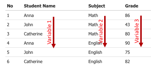
When we arrange each variable in columns and each student in a row then we will get the tidy version of the same data as follows:

No	Student Name	Subject	Grade
1	Anna	Math	86
2	John	Math	43
3	Catherine	Math	80
4	Anna	English	90
5	John	English	75
6	Catherine	English	82

You can see that in this format, each variable forms a column and each student forms a row:

Tidy data

The main advantage of using tidy principles is it allows R’s vectorized nature to shine. One can extract variables in a simple, standard way. Have a look at the following illustration. Which would you rather work with?

Tidy vs. Untidy data

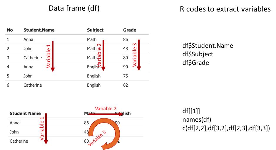
Tidy data is important because the consistent structure lets you focus on questions about the data, not fighting to get the data into the right form for different functions.

Common problems with messy data sets

Real data sets can, and often do, violate the three principles of tidy data. This section describes most common problems with messy datasets:

Column headers are values, not variable names: A common problem is a dataset where some (or all) of the column names are not names of variables, but values of a variable. Here is an illustration of this problem:

Tidy data

In the example above, the column names 2011, 2012, and 2013 represent values of the year variable, and each row represents three observations, not one.

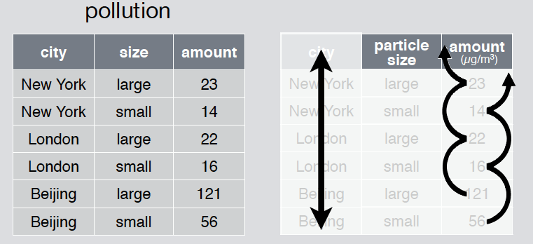
Multiple variables are stored in rows: The opposite of the first problem can also occur when the variables are stored in rows. In such cases, cells include the actual variables, not the observations. Here is an example:

Tidy data

Multiple variables are stored in one column: Sometimes, one column stores the information of two or more variables. Therefore, multiple variables can be extracted from one column. Here is an illustration of this problem:

Tidy data

In the example above, date variable actually stores three new variable information, namely; year, month, and day.

Multiple columns forms a variable: You may need to combine multiple columns into a single column to form a new variable. Here is an illustration of this problem:

Tidy data

In this example, the year, month, and day variables are given separately in the original data but assume that we need to combine these three columns into a single variable called date for the time series analysis.

The `tidyr` package

Most messy datasets can be tidied with a small set of tools. The tidyr package is a very useful package that reshapes the layout of data sets. In the next section you will be introduced the tidyr package and its functions with examples.

We will use the subset of the data contained in the World Health Organization Global Tuberculosis Report (also given in tidyr package documentation) to illustrate the functions in the tidyr package. Before loading this dataset, we need to install and load the package using:

# install the tidyr package

#install.packages("tidyr")

# load the tidyr package

library(tidyr)

The following example shows the same data organized in four different ways (table1, table2, table3, table4a, table4b). Each dataset shows the same values of four variables, country, year, population, and cases, but each dataset organizes the values in a different way as follows:

# load the example data organized in four different ways

table1

## # A tibble: 6 × 4
##   country      year  cases population
##   <chr>       <dbl>  <dbl>      <dbl>
## 1 Afghanistan  1999    745   19987071
## 2 Afghanistan  2000   2666   20595360
## 3 Brazil       1999  37737  172006362
## 4 Brazil       2000  80488  174504898
## 5 China        1999 212258 1272915272
## 6 China        2000 213766 1280428583

table2

## # A tibble: 12 × 4
##    country      year type            count
##    <chr>       <dbl> <chr>           <dbl>
##  1 Afghanistan  1999 cases             745
##  2 Afghanistan  1999 population   19987071
##  3 Afghanistan  2000 cases            2666
##  4 Afghanistan  2000 population   20595360
##  5 Brazil       1999 cases           37737
##  6 Brazil       1999 population  172006362
##  7 Brazil       2000 cases           80488
##  8 Brazil       2000 population  174504898
##  9 China        1999 cases          212258
## 10 China        1999 population 1272915272
## 11 China        2000 cases          213766
## 12 China        2000 population 1280428583

table3

## # A tibble: 6 × 3
##   country      year rate             
##   <chr>       <dbl> <chr>            
## 1 Afghanistan  1999 745/19987071     
## 2 Afghanistan  2000 2666/20595360    
## 3 Brazil       1999 37737/172006362  
## 4 Brazil       2000 80488/174504898  
## 5 China        1999 212258/1272915272
## 6 China        2000 213766/1280428583

table4a

## # A tibble: 3 × 3
##   country     `1999` `2000`
##   <chr>        <dbl>  <dbl>
## 1 Afghanistan    745   2666
## 2 Brazil       37737  80488
## 3 China       212258 213766

table4b

## # A tibble: 3 × 3
##   country         `1999`     `2000`
##   <chr>            <dbl>      <dbl>
## 1 Afghanistan   19987071   20595360
## 2 Brazil       172006362  174504898
## 3 China       1272915272 1280428583

`pivot_longer()` function

The function pivot_longer() is an updated approach to gather() function. When column names are values instead of variables, we need to gather or in other words, we need to transform data from wide to long format.

Fig2. gather() – tidyr by RStudio

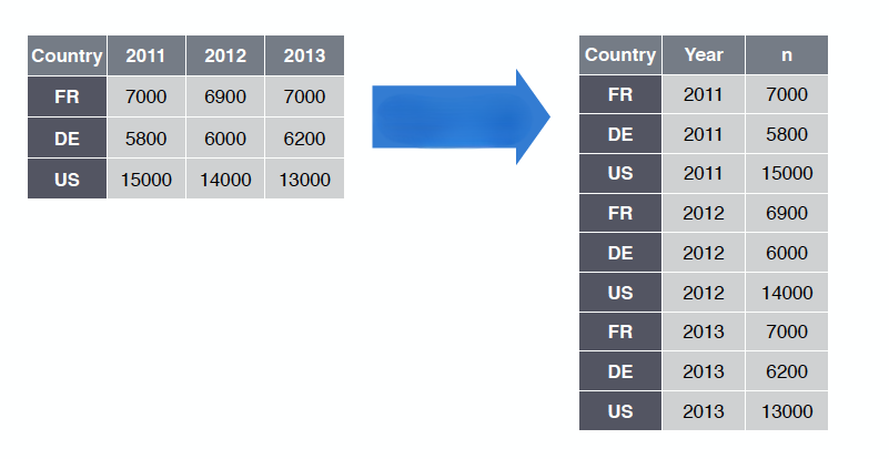
To illustrate gather() function, let’s have a look at the data given in table4a:

table4a

## # A tibble: 3 × 3
##   country     `1999` `2000`
##   <chr>        <dbl>  <dbl>
## 1 Afghanistan    745   2666
## 2 Brazil       37737  80488
## 3 China       212258 213766

To tidy a dataset like this, we need to gather those columns into a new pair of variables using gather() function. To describe that operation, we need three parameters:

The set of columns that represent values, not variables. In this example, those are the columns 1999 and 2000.
The name of the variable whose values form the column names. The argument name key stands for that variable. For this example, the key argument is year.
The name of the variable whose values are spread over the cells. The argument name value stands for that, in this example value argument is the number of cases.

table4a %>% gather(`1999`, `2000`, key = "year", value = "cases")

## # A tibble: 6 × 3
##   country     year   cases
##   <chr>       <chr>  <dbl>
## 1 Afghanistan 1999     745
## 2 Brazil      1999   37737
## 3 China       1999  212258
## 4 Afghanistan 2000    2666
## 5 Brazil      2000   80488
## 6 China       2000  213766

OR using the pivot_longer function:

table4a %>% pivot_longer(names_to = "year", values_to = "cases", cols = 2:3)

## # A tibble: 6 × 3
##   country     year   cases
##   <chr>       <chr>  <dbl>
## 1 Afghanistan 1999     745
## 2 Afghanistan 2000    2666
## 3 Brazil      1999   37737
## 4 Brazil      2000   80488
## 5 China       1999  212258
## 6 China       2000  213766

Here, the arguments names_to is a string specifying the name of the column to create from the data stored in the column names of data, values_to is a string specifying the name of the column to create from the data stored in cell values, and cols refers to those columns that should be pivot into longer format.

Note that in the R code below, I used the pipe (%>%) operator to take the data first, then use the gather function. The tidyr package functions can also be used along with the pipe operator %>% which is developed by Stefan Milton Bache in the R package magrittr. Remember that the functions in tidyr can be used without the pipe operator. For more information on the pipe operator, its pros and cons please refer to Dr. James Baglin’s R Bootcamp Course 1.

`pivot_wider()` function

The function pivot_wider() is an updated approach to spread() function. When multiple variables are stored in rows, the spread() function generates columns from rows. In other words, it transforms data from long to wide format. The spread() function is the opposite of gather() function.

Fig3. spread() – tidyr by RStudio

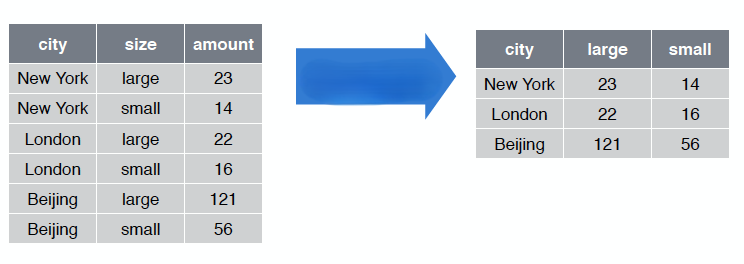
Let’s look at table2 and assume that we are required to turn long formatted data into wide formatted data by generating columns from cases.

table2

## # A tibble: 12 × 4
##    country      year type            count
##    <chr>       <dbl> <chr>           <dbl>
##  1 Afghanistan  1999 cases             745
##  2 Afghanistan  1999 population   19987071
##  3 Afghanistan  2000 cases            2666
##  4 Afghanistan  2000 population   20595360
##  5 Brazil       1999 cases           37737
##  6 Brazil       1999 population  172006362
##  7 Brazil       2000 cases           80488
##  8 Brazil       2000 population  174504898
##  9 China        1999 cases          212258
## 10 China        1999 population 1272915272
## 11 China        2000 cases          213766
## 12 China        2000 population 1280428583

To tidy this up, we first analyse the representation in a similar way to gather(). This time, however, we only need two parameters:

The column that contains variable names, the key column. Here, it’s type.
The column that contains values from multiple variables, the value column. Here, it’s count.

Once we’ve figured that out, we can use spread():

spread(table2, key = "type", value = "count")

## # A tibble: 6 × 4
##   country      year  cases population
##   <chr>       <dbl>  <dbl>      <dbl>
## 1 Afghanistan  1999    745   19987071
## 2 Afghanistan  2000   2666   20595360
## 3 Brazil       1999  37737  172006362
## 4 Brazil       2000  80488  174504898
## 5 China        1999 212258 1272915272
## 6 China        2000 213766 1280428583

OR equivalently, we have the following using the function pivot_wider() with the arguments names_from and values_from:

pivot_wider(table2, names_from = "type", values_from = "count")

## # A tibble: 6 × 4
##   country      year  cases population
##   <chr>       <dbl>  <dbl>      <dbl>
## 1 Afghanistan  1999    745   19987071
## 2 Afghanistan  2000   2666   20595360
## 3 Brazil       1999  37737  172006362
## 4 Brazil       2000  80488  174504898
## 5 China        1999 212258 1272915272
## 6 China        2000 213766 1280428583

Now, cases and population are separate variables given in columns, therefore, generating a new variable from these two variables is super easy! Let’s calculate the Tuberculosis rate (rate = cases/population) using:

rate = spread(table2, key = type, value = count)$cases / spread(table2, key = type, value = count)$population

rate

## [1] 0.0000372741 0.0001294466 0.0002193930 0.0004612363 0.0001667495
## [6] 0.0001669488

`separate()` function

The separate() and extract() functions both can be used when multiple variables are stored in one column and you want to split them according to the separator character. Take table3 for example:

table3

## # A tibble: 6 × 3
##   country      year rate             
##   <chr>       <dbl> <chr>            
## 1 Afghanistan  1999 745/19987071     
## 2 Afghanistan  2000 2666/20595360    
## 3 Brazil       1999 37737/172006362  
## 4 Brazil       2000 80488/174504898  
## 5 China        1999 212258/1272915272
## 6 China        2000 213766/1280428583

The rate column contains both cases and population variables, and we need to split it into two variables.

table3 %>% separate(rate, into = c("cases", "population"), sep = "/")

## # A tibble: 6 × 4
##   country      year cases  population
##   <chr>       <dbl> <chr>  <chr>     
## 1 Afghanistan  1999 745    19987071  
## 2 Afghanistan  2000 2666   20595360  
## 3 Brazil       1999 37737  172006362 
## 4 Brazil       2000 80488  174504898 
## 5 China        1999 212258 1272915272
## 6 China        2000 213766 1280428583

`unite()` function

unite() is the inverse of separate() function. One can use it to combine multiple columns into a single column.

Now let’s look at this data:

table5

## # A tibble: 6 × 4
##   country     century year  rate             
##   <chr>       <chr>   <chr> <chr>            
## 1 Afghanistan 19      99    745/19987071     
## 2 Afghanistan 20      00    2666/20595360    
## 3 Brazil      19      99    37737/172006362  
## 4 Brazil      20      00    80488/174504898  
## 5 China       19      99    212258/1272915272
## 6 China       20      00    213766/1280428583

In this data, assume that we want to combine the century and year variables into one variable called new_year. We can use unite() for this purpose:

table5 %>% unite(new_year, century, year)

## # A tibble: 6 × 3
##   country     new_year rate             
##   <chr>       <chr>    <chr>            
## 1 Afghanistan 19_99    745/19987071     
## 2 Afghanistan 20_00    2666/20595360    
## 3 Brazil      19_99    37737/172006362  
## 4 Brazil      20_00    80488/174504898  
## 5 China       19_99    212258/1272915272
## 6 China       20_00    213766/1280428583

In this case we also need to use the sep argument. The default will place an underscore (_) between the values from different columns. Here we don’t want any separator, so we use sep="" as follows:

table5 %>% unite(new_year, century, year, sep="")

## # A tibble: 6 × 3
##   country     new_year rate             
##   <chr>       <chr>    <chr>            
## 1 Afghanistan 1999     745/19987071     
## 2 Afghanistan 2000     2666/20595360    
## 3 Brazil      1999     37737/172006362  
## 4 Brazil      2000     80488/174504898  
## 5 China       1999     212258/1272915272
## 6 China       2000     213766/1280428583

The `dplyr` package

Although there are many data manipulation packages/functions in R, most of them lack consistent coding and the ability to easily flow together. This leads to difficult-to-read nested functions and/or choppy code. Hadley Wickham developed the very popular dplyr package to make these data processing tasks more efficient along with a syntax that is consistent and easier to remember and read.

The dplyr package is regarded as the “Grammar of Data Manipulation” in R and it originates from the popular plyr package, also developed by Hadley Wickham. The plyr package covers data manipulation for a range of data structures (i.e., data frames, lists, arrays) whereas dplyr is focused on data frames. In this section, I will focus on dplyr. We will cover primary functions inside dplyr for data manipulation. The full list of capabilities can be found in the dplyr reference manual. I highly recommend going through it as there are many great functions provided by dplyr that I will not cover here.

I will use the nycflights13 package and the data sets to explore the basic data manipulation verbs of dplyr. First, we need to install and load the dplyr and nycflights13 packages using:

# install the dplyr package

#install.packages("dplyr")

# load the dplyr package

library(dplyr)

# install the nycflights13 package for the data set

#install.packages("nycflights13")

# load the nycflights13 package

library(nycflights13)

The nycflights13 package includes five data frames containing information on airlines, airports, flights, weather, and planes that departed from New York City in 2013. The data comes from the US Bureau of Transportation Statistics. Let’s look at the nycflights13::flights data set:

# View the flights data set under the nycflights13 package

nycflights13::flights

## # A tibble: 336,776 × 19
##     year month   day dep_time sched_dep_time dep_delay arr_time sched_arr_time
##    <int> <int> <int>    <int>          <int>     <dbl>    <int>          <int>
##  1  2013     1     1      517            515         2      830            819
##  2  2013     1     1      533            529         4      850            830
##  3  2013     1     1      542            540         2      923            850
##  4  2013     1     1      544            545        -1     1004           1022
##  5  2013     1     1      554            600        -6      812            837
##  6  2013     1     1      554            558        -4      740            728
##  7  2013     1     1      555            600        -5      913            854
##  8  2013     1     1      557            600        -3      709            723
##  9  2013     1     1      557            600        -3      838            846
## 10  2013     1     1      558            600        -2      753            745
## # ℹ 336,766 more rows
## # ℹ 11 more variables: arr_delay <dbl>, carrier <chr>, flight <int>,
## #   tailnum <chr>, origin <chr>, dest <chr>, air_time <dbl>, distance <dbl>,
## #   hour <dbl>, minute <dbl>, time_hour <dttm>

You might notice that this data frame prints differently from other data frames you might have used in the past: it only shows the first few rows and all the columns that fit on one screen. It prints differently because it’s a tibble. Tibbles are a modern take on data frames. They are slightly tweaked to work better with tidyr and dplyr (and many others). For now, you don’t need to worry about the differences (you may refer to here to learn more on tibbles.

`select()` function

When working with a large data frame, often we want to only assess specific variables. The select() function allows us to select and/or rename variables.

In addition to the existing functions like : and c(), there are a number of special functions that can work inside select. Some of them are given in the following table.

Functions	Usage
`-`	Select everything but
`:`	Select range
`contains()`	Select columns whose name contains a character string
`ends_with()`	Select columns whose name ends with a string
`everything()`	Select every column
`matches()`	Select columns whose name matches a regular expression
`num_range()`	Select columns named x1, x2, x3, x4, x5
`one_of()`	Select columns whose names are in a group of names
`starts_with()`	Select columns whose name starts with a character string

To illustrate we will use the flights data. Let’s select year, month and day columns using:

# Select columns: year, month and day

dplyr::select(flights, year, month, day)

## # A tibble: 336,776 × 3
##     year month   day
##    <int> <int> <int>
##  1  2013     1     1
##  2  2013     1     1
##  3  2013     1     1
##  4  2013     1     1
##  5  2013     1     1
##  6  2013     1     1
##  7  2013     1     1
##  8  2013     1     1
##  9  2013     1     1
## 10  2013     1     1
## # ℹ 336,766 more rows

Like tidyr, dplyr can also work with the %>% operator. Therefore, we can use the following code to do the same selection:

# Select columns by name using the pipe operator

flights %>%  select(year, month, day)

Here are other examples of using select():

# Select all columns between year and day (inclusive)

flights %>% select(year:day)

## # A tibble: 336,776 × 3
##     year month   day
##    <int> <int> <int>
##  1  2013     1     1
##  2  2013     1     1
##  3  2013     1     1
##  4  2013     1     1
##  5  2013     1     1
##  6  2013     1     1
##  7  2013     1     1
##  8  2013     1     1
##  9  2013     1     1
## 10  2013     1     1
## # ℹ 336,766 more rows

# Select all columns except those from year to day (inclusive)

flights %>% select( -(year:day) )

## # A tibble: 336,776 × 16
##    dep_time sched_dep_time dep_delay arr_time sched_arr_time arr_delay carrier
##       <int>          <int>     <dbl>    <int>          <int>     <dbl> <chr>  
##  1      517            515         2      830            819        11 UA     
##  2      533            529         4      850            830        20 UA     
##  3      542            540         2      923            850        33 AA     
##  4      544            545        -1     1004           1022       -18 B6     
##  5      554            600        -6      812            837       -25 DL     
##  6      554            558        -4      740            728        12 UA     
##  7      555            600        -5      913            854        19 B6     
##  8      557            600        -3      709            723       -14 EV     
##  9      557            600        -3      838            846        -8 B6     
## 10      558            600        -2      753            745         8 AA     
## # ℹ 336,766 more rows
## # ℹ 9 more variables: flight <int>, tailnum <chr>, origin <chr>, dest <chr>,
## #   air_time <dbl>, distance <dbl>, hour <dbl>, minute <dbl>, time_hour <dttm>

For more information on available functions in select, type ?select.

`filter()` function

The filter() function allows us to identify or select observations in which a particular variable matches a specific value/condition. The condition in the filter() function can be any kind of logical comparison and Boolean operators, such as:

Symbol	Usage
`<`	Less than
`>`	Greater than
`==`	Equal to
`<=`	Less than or equal to
`>=`	Greater than or equal to
`!=`	Not equal to
`%in%`	Group membership
`is.na`	Is NA
`!is.na`	Is not NA
`&`	Boolean and
`\|`	Boolean or
`xor`	exactly or
`!`	not
`any`	any true
`all`	all true

For example, we can select all flights on January 1st using the following:

# Filter the flights on January 1st

flights %>%  filter( month == 1, day == 1)

## # A tibble: 842 × 19
##     year month   day dep_time sched_dep_time dep_delay arr_time sched_arr_time
##    <int> <int> <int>    <int>          <int>     <dbl>    <int>          <int>
##  1  2013     1     1      517            515         2      830            819
##  2  2013     1     1      533            529         4      850            830
##  3  2013     1     1      542            540         2      923            850
##  4  2013     1     1      544            545        -1     1004           1022
##  5  2013     1     1      554            600        -6      812            837
##  6  2013     1     1      554            558        -4      740            728
##  7  2013     1     1      555            600        -5      913            854
##  8  2013     1     1      557            600        -3      709            723
##  9  2013     1     1      557            600        -3      838            846
## 10  2013     1     1      558            600        -2      753            745
## # ℹ 832 more rows
## # ℹ 11 more variables: arr_delay <dbl>, carrier <chr>, flight <int>,
## #   tailnum <chr>, origin <chr>, dest <chr>, air_time <dbl>, distance <dbl>,
## #   hour <dbl>, minute <dbl>, time_hour <dttm>

When you run that line of code, dplyr executes the filtering operation and returns a new data frame. dplyr functions never modify their inputs, so if you want to save the result, you’ll need to use the assignment operator, <-:

# Filter the flights on January 1st and save this result 

jan1 <- flights %>%  filter( month == 1, day == 1)

The following code finds all flights that departed in November or December:

# Filter the flights departing in November or December

x <- flights %>%  filter( month == 11 | month == 12)

If we want to find flights that aren’t delayed (on arrival or departure) by more than two hours, we can use either of the following two filters:

# Filter the flights that aren't delayed (on arrival or departure) by more than two hours

flights %>% filter( arr_delay <= 120, dep_delay <= 120 )

## # A tibble: 316,050 × 19
##     year month   day dep_time sched_dep_time dep_delay arr_time sched_arr_time
##    <int> <int> <int>    <int>          <int>     <dbl>    <int>          <int>
##  1  2013     1     1      517            515         2      830            819
##  2  2013     1     1      533            529         4      850            830
##  3  2013     1     1      542            540         2      923            850
##  4  2013     1     1      544            545        -1     1004           1022
##  5  2013     1     1      554            600        -6      812            837
##  6  2013     1     1      554            558        -4      740            728
##  7  2013     1     1      555            600        -5      913            854
##  8  2013     1     1      557            600        -3      709            723
##  9  2013     1     1      557            600        -3      838            846
## 10  2013     1     1      558            600        -2      753            745
## # ℹ 316,040 more rows
## # ℹ 11 more variables: arr_delay <dbl>, carrier <chr>, flight <int>,
## #   tailnum <chr>, origin <chr>, dest <chr>, air_time <dbl>, distance <dbl>,
## #   hour <dbl>, minute <dbl>, time_hour <dttm>

# gives the same result as above

flights %>% filter( ! (arr_delay > 120 | dep_delay > 120) )

For more information on available functions in filter, type ?filter.

`arrange()` function

The arrange() function allows us to order data by variables in ascending or descending order.

Let’s order the flights data in an ascending order using year, month and day.

# Order the data set according to three variables

flights %>% arrange( year, month, day )

## # A tibble: 336,776 × 19
##     year month   day dep_time sched_dep_time dep_delay arr_time sched_arr_time
##    <int> <int> <int>    <int>          <int>     <dbl>    <int>          <int>
##  1  2013     1     1      517            515         2      830            819
##  2  2013     1     1      533            529         4      850            830
##  3  2013     1     1      542            540         2      923            850
##  4  2013     1     1      544            545        -1     1004           1022
##  5  2013     1     1      554            600        -6      812            837
##  6  2013     1     1      554            558        -4      740            728
##  7  2013     1     1      555            600        -5      913            854
##  8  2013     1     1      557            600        -3      709            723
##  9  2013     1     1      557            600        -3      838            846
## 10  2013     1     1      558            600        -2      753            745
## # ℹ 336,766 more rows
## # ℹ 11 more variables: arr_delay <dbl>, carrier <chr>, flight <int>,
## #   tailnum <chr>, origin <chr>, dest <chr>, air_time <dbl>, distance <dbl>,
## #   hour <dbl>, minute <dbl>, time_hour <dttm>

We can also apply a descending argument to rank-order from highest to lowest. The following shows the same data but in descending order by applying desc() within the arrange() function.

# Order the data set according to departure time in a descending order

flights %>% arrange( desc(dep_time) )

## # A tibble: 336,776 × 19
##     year month   day dep_time sched_dep_time dep_delay arr_time sched_arr_time
##    <int> <int> <int>    <int>          <int>     <dbl>    <int>          <int>
##  1  2013    10    30     2400           2359         1      327            337
##  2  2013    11    27     2400           2359         1      515            445
##  3  2013    12     5     2400           2359         1      427            440
##  4  2013    12     9     2400           2359         1      432            440
##  5  2013    12     9     2400           2250        70       59           2356
##  6  2013    12    13     2400           2359         1      432            440
##  7  2013    12    19     2400           2359         1      434            440
##  8  2013    12    29     2400           1700       420      302           2025
##  9  2013     2     7     2400           2359         1      432            436
## 10  2013     2     7     2400           2359         1      443            444
## # ℹ 336,766 more rows
## # ℹ 11 more variables: arr_delay <dbl>, carrier <chr>, flight <int>,
## #   tailnum <chr>, origin <chr>, dest <chr>, air_time <dbl>, distance <dbl>,
## #   hour <dbl>, minute <dbl>, time_hour <dttm>

Note that the missing values will always be sorted at the end.

`mutate()` function

The mutate() function allows us to add new variables while preserving the existing variables. Here is the list of some useful functions used inside the mutate().

Functions	Usage
`pmin()`, `pmax()`	Element wise min and max
`cummin()`, `cummax()`	Cumulative min and max
`cumsum()`, `cumprod()`	Cumulative sum and product
`between()`	Are values between a and b?
`cume_dist()`	Cumulative distribution of values
`cumall()`, `cumany()`	Cumulative all and any
`cummean()`	Cumulative mean
`lead()`, `lag()`	Copy with values one position
`ntile()`	Bin vector into n buckets
`dense_rank()`, `min_rank()`, `percent_rank()`, `row_number()`	Various ranking methods

# Select specific variables from the data and store them in a new data frame

flights_sub<- flights %>% select(arr_delay, dep_delay, air_time)


# Create new variables "gain", "hours", and "gain_per_hour"

mutate(flights_sub, gain = arr_delay - dep_delay, hours = air_time / 60, gain_per_hour = gain / hours)

## # A tibble: 336,776 × 6
##    arr_delay dep_delay air_time  gain hours gain_per_hour
##        <dbl>     <dbl>    <dbl> <dbl> <dbl>         <dbl>
##  1        11         2      227     9 3.78           2.38
##  2        20         4      227    16 3.78           4.23
##  3        33         2      160    31 2.67          11.6 
##  4       -18        -1      183   -17 3.05          -5.57
##  5       -25        -6      116   -19 1.93          -9.83
##  6        12        -4      150    16 2.5            6.4 
##  7        19        -5      158    24 2.63           9.11
##  8       -14        -3       53   -11 0.883        -12.5 
##  9        -8        -3      140    -5 2.33          -2.14
## 10         8        -2      138    10 2.3            4.35
## # ℹ 336,766 more rows

Note that the new variables will appear at the end of the flights data frame.

An alternative to mutate() is transmute() which creates a new variable and then drops the other variables. Essentially, it allows you to create a new data frame with only the new variables created.

transmute(flights, gain = arr_delay - dep_delay, hours = air_time / 60, gain_per_hour = gain / hours)

## # A tibble: 336,776 × 3
##     gain hours gain_per_hour
##    <dbl> <dbl>         <dbl>
##  1     9 3.78           2.38
##  2    16 3.78           4.23
##  3    31 2.67          11.6 
##  4   -17 3.05          -5.57
##  5   -19 1.93          -9.83
##  6    16 2.5            6.4 
##  7    24 2.63           9.11
##  8   -11 0.883        -12.5 
##  9    -5 2.33          -2.14
## 10    10 2.3            4.35
## # ℹ 336,766 more rows

`summarise()` (or `summarize()` ) function

The summarise() (a.k.a. summarize() ) function allows us to perform the majority of summary statistics when performing exploratory data analysis. Here is the list of some useful functions that can be used inside summary().

Functions	Usage
`min()`, `max()`	Minimum and maximum values
`mean()`	Mean value
`median()`	Median value
`sum()`	Sum of values
`var()`, `sd()`	Variance and standard deviation of a vector
`first()`	First value in a vector
`last()`	Last value in a vector
`nth()`	Nth value in a vector
`n()`	The number of values in a vector
`n_distinct()`	The number of distinct values in a vector

All functions in this list takes a vector of values and returns a single summary value. We can get the average delay using:

# Take the average of departure delay

summarise(flights, delay = mean(dep_delay, na.rm = TRUE))

## # A tibble: 1 × 1
##   delay
##   <dbl>
## 1  12.6

The na.rm = TRUE argument in mean() function will allow us to ignore the missing values while computing the average. We will revisit na.rm = TRUE argument in the next section (in Module 5).

`group_by()` + `summarise()` function

If we want to take the summary statistics grouped by a variable, then we need to use another function called group_by(). group_by() along with summarise() functions will allow us to take and compare summary statistics grouped by a factor variable.

For example, if we applied the same code to a data frame grouped by destination, we can get the average delay for each destination.

# Group by destination and use summarise to calculate the mean delay

flights %>% group_by(dest) %>% summarise(mean_delay = mean(dep_delay, na.rm = TRUE))

## # A tibble: 105 × 2
##    dest  mean_delay
##    <chr>      <dbl>
##  1 ABQ        13.7 
##  2 ACK         6.46
##  3 ALB        23.6 
##  4 ANC        12.9 
##  5 ATL        12.5 
##  6 AUS        13.0 
##  7 AVL         8.19
##  8 BDL        17.7 
##  9 BGR        19.5 
## 10 BHM        29.7 
## # ℹ 95 more rows

Joining data sets

Often, we have separate data frames that can have common and differing variables for similar observations. These types of data sets are referred as relational data sets.

We will revisit the nycflights13 package. The nycflights13 package contains the following data sets:

airlines includes the names of airline companies and their abbreviated code:

airlines

## # A tibble: 16 × 2
##    carrier name                       
##    <chr>   <chr>                      
##  1 9E      Endeavor Air Inc.          
##  2 AA      American Airlines Inc.     
##  3 AS      Alaska Airlines Inc.       
##  4 B6      JetBlue Airways            
##  5 DL      Delta Air Lines Inc.       
##  6 EV      ExpressJet Airlines Inc.   
##  7 F9      Frontier Airlines Inc.     
##  8 FL      AirTran Airways Corporation
##  9 HA      Hawaiian Airlines Inc.     
## 10 MQ      Envoy Air                  
## 11 OO      SkyWest Airlines Inc.      
## 12 UA      United Air Lines Inc.      
## 13 US      US Airways Inc.            
## 14 VX      Virgin America             
## 15 WN      Southwest Airlines Co.     
## 16 YV      Mesa Airlines Inc.

airports gives information about each airport, identified by the airport code (faa):

airports

## # A tibble: 1,458 × 8
##    faa   name                             lat    lon   alt    tz dst   tzone    
##    <chr> <chr>                          <dbl>  <dbl> <dbl> <dbl> <chr> <chr>    
##  1 04G   Lansdowne Airport               41.1  -80.6  1044    -5 A     America/…
##  2 06A   Moton Field Municipal Airport   32.5  -85.7   264    -6 A     America/…
##  3 06C   Schaumburg Regional             42.0  -88.1   801    -6 A     America/…
##  4 06N   Randall Airport                 41.4  -74.4   523    -5 A     America/…
##  5 09J   Jekyll Island Airport           31.1  -81.4    11    -5 A     America/…
##  6 0A9   Elizabethton Municipal Airport  36.4  -82.2  1593    -5 A     America/…
##  7 0G6   Williams County Airport         41.5  -84.5   730    -5 A     America/…
##  8 0G7   Finger Lakes Regional Airport   42.9  -76.8   492    -5 A     America/…
##  9 0P2   Shoestring Aviation Airfield    39.8  -76.6  1000    -5 U     America/…
## 10 0S9   Jefferson County Intl           48.1 -123.    108    -8 A     America/…
## # ℹ 1,448 more rows

planes gives information about each plane, identified by its tail number (tailnum):

planes

## # A tibble: 3,322 × 9
##    tailnum  year type              manufacturer model engines seats speed engine
##    <chr>   <int> <chr>             <chr>        <chr>   <int> <int> <int> <chr> 
##  1 N10156   2004 Fixed wing multi… EMBRAER      EMB-…       2    55    NA Turbo…
##  2 N102UW   1998 Fixed wing multi… AIRBUS INDU… A320…       2   182    NA Turbo…
##  3 N103US   1999 Fixed wing multi… AIRBUS INDU… A320…       2   182    NA Turbo…
##  4 N104UW   1999 Fixed wing multi… AIRBUS INDU… A320…       2   182    NA Turbo…
##  5 N10575   2002 Fixed wing multi… EMBRAER      EMB-…       2    55    NA Turbo…
##  6 N105UW   1999 Fixed wing multi… AIRBUS INDU… A320…       2   182    NA Turbo…
##  7 N107US   1999 Fixed wing multi… AIRBUS INDU… A320…       2   182    NA Turbo…
##  8 N108UW   1999 Fixed wing multi… AIRBUS INDU… A320…       2   182    NA Turbo…
##  9 N109UW   1999 Fixed wing multi… AIRBUS INDU… A320…       2   182    NA Turbo…
## 10 N110UW   1999 Fixed wing multi… AIRBUS INDU… A320…       2   182    NA Turbo…
## # ℹ 3,312 more rows

weather gives the weather conditions at each NYC airport for each hour:

weather

## # A tibble: 26,115 × 15
##    origin  year month   day  hour  temp  dewp humid wind_dir wind_speed
##    <chr>  <int> <int> <int> <int> <dbl> <dbl> <dbl>    <dbl>      <dbl>
##  1 EWR     2013     1     1     1  39.0  26.1  59.4      270      10.4 
##  2 EWR     2013     1     1     2  39.0  27.0  61.6      250       8.06
##  3 EWR     2013     1     1     3  39.0  28.0  64.4      240      11.5 
##  4 EWR     2013     1     1     4  39.9  28.0  62.2      250      12.7 
##  5 EWR     2013     1     1     5  39.0  28.0  64.4      260      12.7 
##  6 EWR     2013     1     1     6  37.9  28.0  67.2      240      11.5 
##  7 EWR     2013     1     1     7  39.0  28.0  64.4      240      15.0 
##  8 EWR     2013     1     1     8  39.9  28.0  62.2      250      10.4 
##  9 EWR     2013     1     1     9  39.9  28.0  62.2      260      15.0 
## 10 EWR     2013     1     1    10  41    28.0  59.6      260      13.8 
## # ℹ 26,105 more rows
## # ℹ 5 more variables: wind_gust <dbl>, precip <dbl>, pressure <dbl>,
## #   visib <dbl>, time_hour <dttm>

Therefore, for nycflights13:

flights connects to planes via a single variable, tailnum.
flights connects to airlines through the carrier variable.
flights connects to airports in two ways: via the origin and dest variables.
flights connects to weather via origin (the location), and year, month, day, and hour (the time).

The following illustration (adapted from Hadley Wickham, Çetinkaya-Rundel, and Grolemund (2023)) shows the relationship between flights, airlines, airports and weather data sets, and the key variables connecting them.

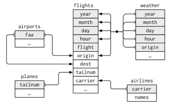
Fig4. Chain of relations between the data sets in nycflights13 (taken from Hadley Wickham, Çetinkaya-Rundel, and Grolemund (2023))

The dplyr package offers three sets of joining functions to provide alternative ways to join data frames. These are:

Mutating joins: This group of functions add new variables to one data frame from matching observations in another.
Filtering joins: This group of functions filter observations from one data frame based on whether or not they match an observation in the other table.
Set operations: This group of functions treat observations as if they were set elements.

Mutating joins

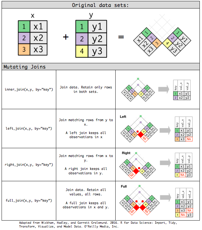
The first set of functions to combine data sets is called “mutating joins”. left_join(), right_join(), inner_join(), and full_join() functions are in this group. The mutating join functions allow you to combine variables from two tables and add variables to the right (like mutate).

Note that, mutating join functions add variables to the right. Therefore, if you have a lot of variables already in the data, the new variables won’t get printed out. As flights data set has many variables, I will first create a narrower data set named flights2 to easily show you what’s going on in the examples.

# Create a new data set named flights2 including year - day, hour, origin, destination, tailnum and carrier variables

flights2 <- flights %>% select(year:day, hour, origin, dest, tailnum, carrier)

flights2

## # A tibble: 336,776 × 8
##     year month   day  hour origin dest  tailnum carrier
##    <int> <int> <int> <dbl> <chr>  <chr> <chr>   <chr>  
##  1  2013     1     1     5 EWR    IAH   N14228  UA     
##  2  2013     1     1     5 LGA    IAH   N24211  UA     
##  3  2013     1     1     5 JFK    MIA   N619AA  AA     
##  4  2013     1     1     5 JFK    BQN   N804JB  B6     
##  5  2013     1     1     6 LGA    ATL   N668DN  DL     
##  6  2013     1     1     5 EWR    ORD   N39463  UA     
##  7  2013     1     1     6 EWR    FLL   N516JB  B6     
##  8  2013     1     1     6 LGA    IAD   N829AS  EV     
##  9  2013     1     1     6 JFK    MCO   N593JB  B6     
## 10  2013     1     1     6 LGA    ORD   N3ALAA  AA     
## # ℹ 336,766 more rows

Imagine you want to add the full airline name (from airlines) to the flights2 data. You can combine the airlines and flights2 data frames using left_join(). Remember that we will need a key variable and the key variable will be the carrier variable to join these two data sets.

# joining flights2 and airlines using the carrier name.

flights2 %>% left_join(airlines, by = "carrier")

## # A tibble: 336,776 × 9
##     year month   day  hour origin dest  tailnum carrier name                    
##    <int> <int> <int> <dbl> <chr>  <chr> <chr>   <chr>   <chr>                   
##  1  2013     1     1     5 EWR    IAH   N14228  UA      United Air Lines Inc.   
##  2  2013     1     1     5 LGA    IAH   N24211  UA      United Air Lines Inc.   
##  3  2013     1     1     5 JFK    MIA   N619AA  AA      American Airlines Inc.  
##  4  2013     1     1     5 JFK    BQN   N804JB  B6      JetBlue Airways         
##  5  2013     1     1     6 LGA    ATL   N668DN  DL      Delta Air Lines Inc.    
##  6  2013     1     1     5 EWR    ORD   N39463  UA      United Air Lines Inc.   
##  7  2013     1     1     6 EWR    FLL   N516JB  B6      JetBlue Airways         
##  8  2013     1     1     6 LGA    IAD   N829AS  EV      ExpressJet Airlines Inc.
##  9  2013     1     1     6 JFK    MCO   N593JB  B6      JetBlue Airways         
## 10  2013     1     1     6 LGA    ORD   N3ALAA  AA      American Airlines Inc.  
## # ℹ 336,766 more rows

Controlling how the data sets are matched

Each mutating join takes an argument by that controls which variables are used to match observations in the two data sets. There are a few ways to specify it:

NULL: The default value. dplyr will use all variables that appear in both tables, a natural join. For example, the flights and weather data sets match on their common variables: year, month, day, hour and origin.

# joining flights2 and weather using the default key = NULL.

flights2 %>% left_join(weather)

## Joining with `by = join_by(year, month, day, hour, origin)`

## # A tibble: 336,776 × 18
##     year month   day  hour origin dest  tailnum carrier  temp  dewp humid
##    <int> <int> <int> <dbl> <chr>  <chr> <chr>   <chr>   <dbl> <dbl> <dbl>
##  1  2013     1     1     5 EWR    IAH   N14228  UA       39.0  28.0  64.4
##  2  2013     1     1     5 LGA    IAH   N24211  UA       39.9  25.0  54.8
##  3  2013     1     1     5 JFK    MIA   N619AA  AA       39.0  27.0  61.6
##  4  2013     1     1     5 JFK    BQN   N804JB  B6       39.0  27.0  61.6
##  5  2013     1     1     6 LGA    ATL   N668DN  DL       39.9  25.0  54.8
##  6  2013     1     1     5 EWR    ORD   N39463  UA       39.0  28.0  64.4
##  7  2013     1     1     6 EWR    FLL   N516JB  B6       37.9  28.0  67.2
##  8  2013     1     1     6 LGA    IAD   N829AS  EV       39.9  25.0  54.8
##  9  2013     1     1     6 JFK    MCO   N593JB  B6       37.9  27.0  64.3
## 10  2013     1     1     6 LGA    ORD   N3ALAA  AA       39.9  25.0  54.8
## # ℹ 336,766 more rows
## # ℹ 7 more variables: wind_dir <dbl>, wind_speed <dbl>, wind_gust <dbl>,
## #   precip <dbl>, pressure <dbl>, visib <dbl>, time_hour <dttm>

A character vector, by = "x". For example, flights and planes have tailnum in common.

# joining flights2 and planes using the tailnum.

flights2 %>% left_join(planes, by = "tailnum")

## # A tibble: 336,776 × 16
##    year.x month   day  hour origin dest  tailnum carrier year.y type            
##     <int> <int> <int> <dbl> <chr>  <chr> <chr>   <chr>    <int> <chr>           
##  1   2013     1     1     5 EWR    IAH   N14228  UA        1999 Fixed wing mult…
##  2   2013     1     1     5 LGA    IAH   N24211  UA        1998 Fixed wing mult…
##  3   2013     1     1     5 JFK    MIA   N619AA  AA        1990 Fixed wing mult…
##  4   2013     1     1     5 JFK    BQN   N804JB  B6        2012 Fixed wing mult…
##  5   2013     1     1     6 LGA    ATL   N668DN  DL        1991 Fixed wing mult…
##  6   2013     1     1     5 EWR    ORD   N39463  UA        2012 Fixed wing mult…
##  7   2013     1     1     6 EWR    FLL   N516JB  B6        2000 Fixed wing mult…
##  8   2013     1     1     6 LGA    IAD   N829AS  EV        1998 Fixed wing mult…
##  9   2013     1     1     6 JFK    MCO   N593JB  B6        2004 Fixed wing mult…
## 10   2013     1     1     6 LGA    ORD   N3ALAA  AA          NA <NA>            
## # ℹ 336,766 more rows
## # ℹ 6 more variables: manufacturer <chr>, model <chr>, engines <int>,
## #   seats <int>, speed <int>, engine <chr>

A named character vector: by = c("a" = "b"). This will match variable a in table x to variable b in table y. This is useful when the key variables in both data sets are not given the same name. For example, flights data set has the destination airport code (dest) and the airports data set has the faa code. Essentially these two are equivalent. Therefore, we can use the following to join these two data sets:

flights2 %>% left_join(airports, c("dest" = "faa"))

## # A tibble: 336,776 × 15
##     year month   day  hour origin dest  tailnum carrier name     lat   lon   alt
##    <int> <int> <int> <dbl> <chr>  <chr> <chr>   <chr>   <chr>  <dbl> <dbl> <dbl>
##  1  2013     1     1     5 EWR    IAH   N14228  UA      Georg…  30.0 -95.3    97
##  2  2013     1     1     5 LGA    IAH   N24211  UA      Georg…  30.0 -95.3    97
##  3  2013     1     1     5 JFK    MIA   N619AA  AA      Miami…  25.8 -80.3     8
##  4  2013     1     1     5 JFK    BQN   N804JB  B6      <NA>    NA    NA      NA
##  5  2013     1     1     6 LGA    ATL   N668DN  DL      Harts…  33.6 -84.4  1026
##  6  2013     1     1     5 EWR    ORD   N39463  UA      Chica…  42.0 -87.9   668
##  7  2013     1     1     6 EWR    FLL   N516JB  B6      Fort …  26.1 -80.2     9
##  8  2013     1     1     6 LGA    IAD   N829AS  EV      Washi…  38.9 -77.5   313
##  9  2013     1     1     6 JFK    MCO   N593JB  B6      Orlan…  28.4 -81.3    96
## 10  2013     1     1     6 LGA    ORD   N3ALAA  AA      Chica…  42.0 -87.9   668
## # ℹ 336,766 more rows
## # ℹ 3 more variables: tz <dbl>, dst <chr>, tzone <chr>

To help you learn how different types of xxx_join() functions work, I’m going to use Hadley Wickham’s visual representation (Hadley Wickham, Çetinkaya-Rundel, and Grolemund (2023)):

Mutating Joins

Filtering Joins

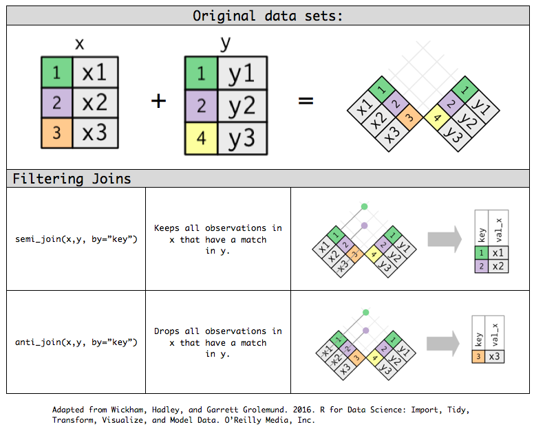
Filtering joins match observations in the same way as mutating joins, but affect the observations, not the variables. There are two types of filtering joins: semi_join() and anti_join().

semi_join(x, y): keeps all observations in x that have a match in y.
anti_join(x, y): drops all observations in x that have a match in y.

Anti-joins are useful for diagnosing join mismatches. For example, when connecting flights and planes, you might be interested to know that there are many flights that don’t have a match in planes:

flights %>% anti_join(planes, by = "tailnum") %>% count(tailnum, sort = TRUE)

## # A tibble: 722 × 2
##    tailnum     n
##    <chr>   <int>
##  1 <NA>     2512
##  2 N725MQ    575
##  3 N722MQ    513
##  4 N723MQ    507
##  5 N713MQ    483
##  6 N735MQ    396
##  7 N0EGMQ    371
##  8 N534MQ    364
##  9 N542MQ    363
## 10 N531MQ    349
## # ℹ 712 more rows

Here is a visual representation of these two filtering joins.

Filtering Joins

When to use mutating or filtering joins

Suppose you have flights2 (X) and weather (Y) data sets. Recall, these data sets match on their common variables: year, month, day, hour and origin.

If you want to add/combine columns to/from data set X from/to data set Y, you need to use mutating joins.

LEFT_JOIN: Let’s say, you want to see the weather of flights departing at 6 in the morning. You will need to use left_join() to ADD the weather columns to the flights2 data set.

flights2_h6 <- flights2 %>% filter(hour == 6)

# joining flights2 and weather using the default key = NULL.
flights2_h6 %>% left_join(weather)

## Joining with `by = join_by(year, month, day, hour, origin)`

## # A tibble: 25,951 × 18
##     year month   day  hour origin dest  tailnum carrier  temp  dewp humid
##    <int> <int> <int> <dbl> <chr>  <chr> <chr>   <chr>   <dbl> <dbl> <dbl>
##  1  2013     1     1     6 LGA    ATL   N668DN  DL       39.9  25.0  54.8
##  2  2013     1     1     6 EWR    FLL   N516JB  B6       37.9  28.0  67.2
##  3  2013     1     1     6 LGA    IAD   N829AS  EV       39.9  25.0  54.8
##  4  2013     1     1     6 JFK    MCO   N593JB  B6       37.9  27.0  64.3
##  5  2013     1     1     6 LGA    ORD   N3ALAA  AA       39.9  25.0  54.8
##  6  2013     1     1     6 JFK    PBI   N793JB  B6       37.9  27.0  64.3
##  7  2013     1     1     6 JFK    TPA   N657JB  B6       37.9  27.0  64.3
##  8  2013     1     1     6 JFK    LAX   N29129  UA       37.9  27.0  64.3
##  9  2013     1     1     6 EWR    SFO   N53441  UA       37.9  28.0  67.2
## 10  2013     1     1     6 LGA    DFW   N3DUAA  AA       39.9  25.0  54.8
## # ℹ 25,941 more rows
## # ℹ 7 more variables: wind_dir <dbl>, wind_speed <dbl>, wind_gust <dbl>,
## #   precip <dbl>, pressure <dbl>, visib <dbl>, time_hour <dttm>

RIGHT_JOIN: Let’s say, you want to see the flights that has weather visibility of 5. You will need to use right_join() to ADD the flights2 columns to the weather data set.

weather_v5 <- weather %>% filter(visib == 5)

flights2 %>% right_join(weather_v5) %>% select(visib, everything())

## Joining with `by = join_by(year, month, day, hour, origin)`

## # A tibble: 4,916 × 18
##    visib  year month   day  hour origin dest  tailnum carrier  temp  dewp humid
##    <dbl> <int> <int> <int> <dbl> <chr>  <chr> <chr>   <chr>   <dbl> <dbl> <dbl>
##  1     5  2013     1     9     7 LGA    BOS   N947UW  US       37.0  33.1  85.4
##  2     5  2013     1     9     7 LGA    DCA   N712US  US       37.0  33.1  85.4
##  3     5  2013     1     9     7 LGA    MIA   N953DL  DL       37.0  33.1  85.4
##  4     5  2013     1     9     7 LGA    ORD   N466AA  AA       37.0  33.1  85.4
##  5     5  2013     1     9     7 LGA    MIA   N3CDAA  AA       37.0  33.1  85.4
##  6     5  2013     1     9     7 LGA    XNA   N730MQ  MQ       37.0  33.1  85.4
##  7     5  2013     1     9     7 LGA    ORD   N438UA  UA       37.0  33.1  85.4
##  8     5  2013     1     9     7 LGA    MCO   N506JB  B6       37.0  33.1  85.4
##  9     5  2013     1     9     7 LGA    MKE   N979AT  FL       37.0  33.1  85.4
## 10     5  2013     1     9     7 LGA    RSW   N593JB  B6       37.0  33.1  85.4
## # ℹ 4,906 more rows
## # ℹ 6 more variables: wind_dir <dbl>, wind_speed <dbl>, wind_gust <dbl>,
## #   precip <dbl>, pressure <dbl>, time_hour <dttm>

INNER_JOIN: Let’s say, you want to see the flights that departs at 6 in the morning and has weather visibility of 5. You will need to use inner_join() to COMBINE the flights2_h6 and weather_v5 columns into a single data set with hour = 6 and visib = 5.

flights2_h6 %>% inner_join(weather_v5) %>% select(hour, visib, everything())

## Joining with `by = join_by(year, month, day, hour, origin)`

## # A tibble: 497 × 18
##     hour visib  year month   day origin dest  tailnum carrier  temp  dewp humid
##    <dbl> <dbl> <int> <int> <int> <chr>  <chr> <chr>   <chr>   <dbl> <dbl> <dbl>
##  1     6     5  2013     1    29 JFK    FLL   N588JB  B6       37.0  35.1  92.5
##  2     6     5  2013     1    29 JFK    IAD   N830AS  EV       37.0  35.1  92.5
##  3     6     5  2013     1    29 JFK    RSW   N516JB  B6       37.0  35.1  92.5
##  4     6     5  2013     1    29 JFK    PHL   N949UW  US       37.0  35.1  92.5
##  5     6     5  2013     1    29 JFK    LAX   N67134  UA       37.0  35.1  92.5
##  6     6     5  2013     1    29 JFK    SFO   N532UA  UA       37.0  35.1  92.5
##  7     6     5  2013     1    29 JFK    PBI   N768JB  B6       37.0  35.1  92.5
##  8     6     5  2013     1    29 JFK    SJU   N793JB  B6       37.0  35.1  92.5
##  9     6     5  2013     1    29 JFK    ATL   N197PQ  9E       37.0  35.1  92.5
## 10     6     5  2013     1    29 JFK    BOS   N775JB  B6       37.0  35.1  92.5
## # ℹ 487 more rows
## # ℹ 6 more variables: wind_dir <dbl>, wind_speed <dbl>, wind_gust <dbl>,
## #   precip <dbl>, pressure <dbl>, time_hour <dttm>

FULL_JOIN: Let’s say, you want to see the flights that departs at 6 in the morning or has weather visibility of 5. You will need to use full_join() to COMBINE the flights2_h6 and weather_v5 columns into a single data set with hour = 6 OR visib = 5.

flights2_h6 %>% full_join(weather_v5) %>% select(hour, visib, everything())

## Joining with `by = join_by(year, month, day, hour, origin)`

## # A tibble: 26,315 × 18
##     hour visib  year month   day origin dest  tailnum carrier  temp  dewp humid
##    <dbl> <dbl> <int> <int> <int> <chr>  <chr> <chr>   <chr>   <dbl> <dbl> <dbl>
##  1     6    NA  2013     1     1 LGA    ATL   N668DN  DL         NA    NA    NA
##  2     6    NA  2013     1     1 EWR    FLL   N516JB  B6         NA    NA    NA
##  3     6    NA  2013     1     1 LGA    IAD   N829AS  EV         NA    NA    NA
##  4     6    NA  2013     1     1 JFK    MCO   N593JB  B6         NA    NA    NA
##  5     6    NA  2013     1     1 LGA    ORD   N3ALAA  AA         NA    NA    NA
##  6     6    NA  2013     1     1 JFK    PBI   N793JB  B6         NA    NA    NA
##  7     6    NA  2013     1     1 JFK    TPA   N657JB  B6         NA    NA    NA
##  8     6    NA  2013     1     1 JFK    LAX   N29129  UA         NA    NA    NA
##  9     6    NA  2013     1     1 EWR    SFO   N53441  UA         NA    NA    NA
## 10     6    NA  2013     1     1 LGA    DFW   N3DUAA  AA         NA    NA    NA
## # ℹ 26,305 more rows
## # ℹ 6 more variables: wind_dir <dbl>, wind_speed <dbl>, wind_gust <dbl>,
## #   precip <dbl>, pressure <dbl>, time_hour <dttm>

Meanwhile, if you want to filter records in data set X using data set Y retaining only columns of data set X, you need to use filtering joins.

SEMI_JOIN: Let’s say, you want to see flights with weather visibility of 5. You will need to use semi_join() to FILTER the flights2 data set using the weather_v5 data set.

flights2 %>% semi_join(weather_v5)

## Joining with `by = join_by(year, month, day, hour, origin)`

## # A tibble: 4,809 × 8
##     year month   day  hour origin dest  tailnum carrier
##    <int> <int> <int> <dbl> <chr>  <chr> <chr>   <chr>  
##  1  2013     1     9     7 LGA    BOS   N947UW  US     
##  2  2013     1     9     7 LGA    DCA   N712US  US     
##  3  2013     1     9     7 LGA    MIA   N953DL  DL     
##  4  2013     1     9     7 LGA    ORD   N466AA  AA     
##  5  2013     1     9     7 LGA    MIA   N3CDAA  AA     
##  6  2013     1     9     7 LGA    XNA   N730MQ  MQ     
##  7  2013     1     9     7 LGA    ORD   N438UA  UA     
##  8  2013     1     9     7 LGA    MCO   N506JB  B6     
##  9  2013     1     9     7 LGA    MKE   N979AT  FL     
## 10  2013     1     9     7 LGA    RSW   N593JB  B6     
## # ℹ 4,799 more rows

ANTI_JOIN: Let’s say, you want to see flights with weather visibility not equal to 5. You will need to use anti_join() to FILTER the flights2 data set using the weather_v5 dataset.

flights2 %>% anti_join(weather_v5)

## Joining with `by = join_by(year, month, day, hour, origin)`

## # A tibble: 331,967 × 8
##     year month   day  hour origin dest  tailnum carrier
##    <int> <int> <int> <dbl> <chr>  <chr> <chr>   <chr>  
##  1  2013     1     1     5 EWR    IAH   N14228  UA     
##  2  2013     1     1     5 LGA    IAH   N24211  UA     
##  3  2013     1     1     5 JFK    MIA   N619AA  AA     
##  4  2013     1     1     5 JFK    BQN   N804JB  B6     
##  5  2013     1     1     6 LGA    ATL   N668DN  DL     
##  6  2013     1     1     5 EWR    ORD   N39463  UA     
##  7  2013     1     1     6 EWR    FLL   N516JB  B6     
##  8  2013     1     1     6 LGA    IAD   N829AS  EV     
##  9  2013     1     1     6 JFK    MCO   N593JB  B6     
## 10  2013     1     1     6 LGA    ORD   N3ALAA  AA     
## # ℹ 331,957 more rows

Set operations

Set operations expect the x and y inputs to have the same variables and treat the observations like sets. There are three types of set operations:

intersect(x, y): return only observations in both x and y.
union(x, y): return unique observations in x and y.
setdiff(x, y): return observations in x, but not in y.

Set operators

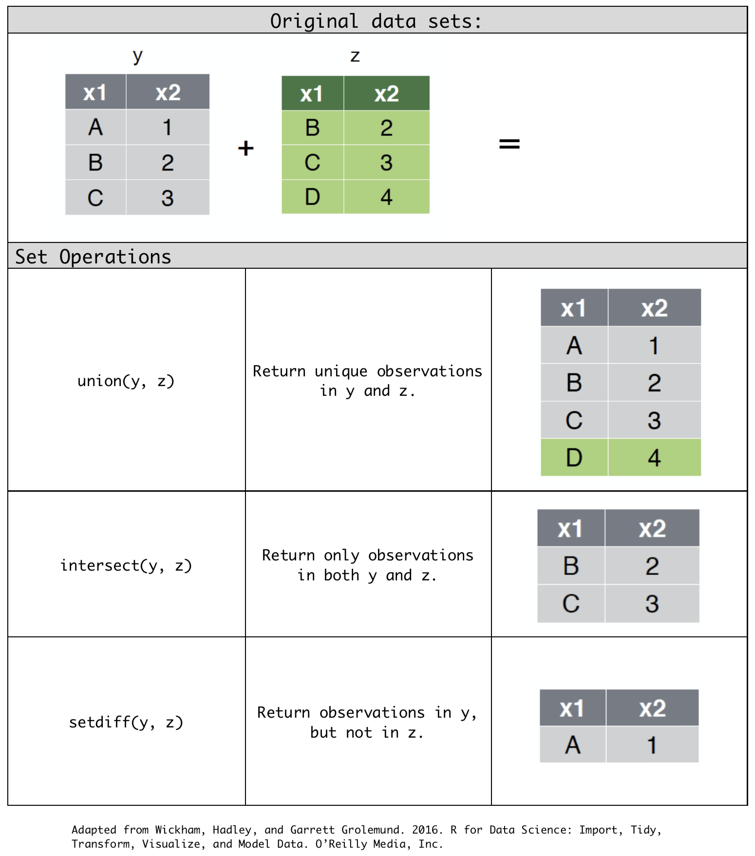
Merging data sets

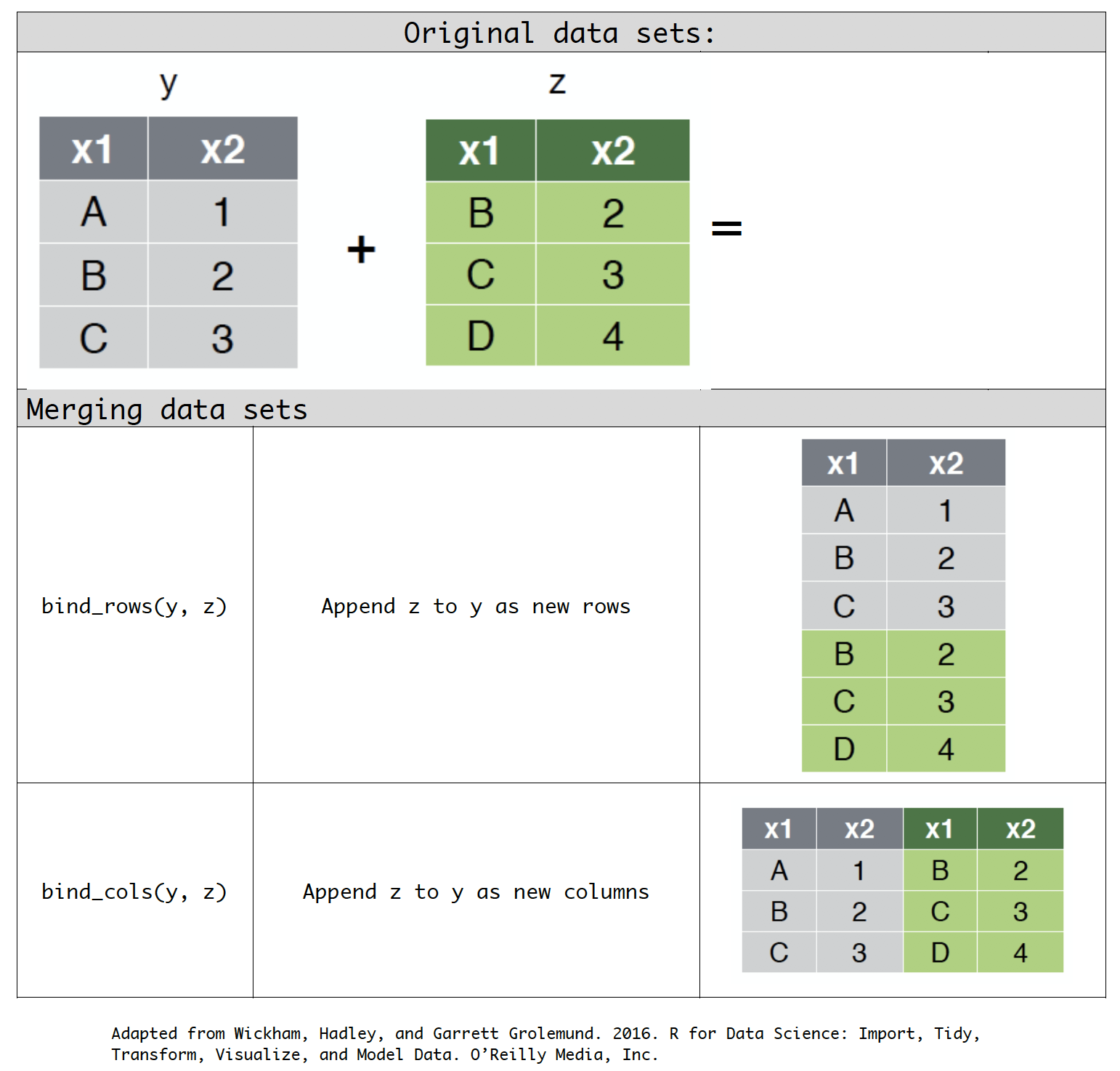
Often you may just need to merge data frames by row and column. The bind_rows() and bind_cols() bind the multiple data frames by row and column, respectively.

bind_rows(x, y): Append y to x as new rows.
bind_cols(x, y): Append y to x as new columns.

Merging Data sets

Additional Resources and Further Reading

You can refer to the tidyr package manual (H. Wickham (2024)) and the Tidy Data paper for a detailed information on tidy data principles and tidyr package.

Our recommended textbooks (Boehmke (2016) and Hadley Wickham, Çetinkaya-Rundel, and Grolemund (2023)), R Studio’s Data wrangling with R and RStudio webinar, and dplyr reference manual (H. Wickham (2024), H. Wickham et al. (2023)) are great resources to excel your knowledge in Data Manipulation with dplyr.

If you are interested in improving your coding style, I would recommend using the tidyverse style guide. Note that a good coding style is like correct punctuation, you can manage without it, but a good coding style makes things easier to read for you and for the others who are gonna use your codes!

References

Boehmke, Bradley C. 2016. Data Wrangling with r. Springer.

Wickham, H. 2024. “Tidyr: Easily Tidy Data with Spread () and Gather () Functions. R Package.” Version 1.3.1 Available at Http://CRAN. R-Project. Org/Package= Tidyr [Verified 22 January 2025].

Wickham, Hadley et al. 2014. “Tidy Data.” Journal of Statistical Software 59 (10): 1–23.

Wickham, Hadley, Mine Çetinkaya-Rundel, and Garrett Grolemund. 2023. R for Data Science. " O’Reilly Media, Inc.".

Wickham, H, R Francois, L Henry, and K Müller. 2023. “Dplyr: A Grammar of Data Manipulation. R Package Version 0.7. 0.” Version 1.1.4 Available at https://cran.r-project.org/web/packages/dplyr/dplyr.pdf.

Module 4

Tidy and Manipulate: Tidy Data Principles and Manipulating Data

Overview

Summary

Learning Objectives

Tidy Data Principles

Common problems with messy data sets

The `tidyr` package

`pivot_longer()` function

`pivot_wider()` function

`separate()` function

`unite()` function

The `dplyr` package

`select()` function

`filter()` function

`arrange()` function

`mutate()` function

`summarise()` (or `summarize()` ) function

`group_by()` + `summarise()` function

Joining data sets

Mutating joins

Controlling how the data sets are matched

Filtering Joins

When to use mutating or filtering joins

Set operations

Merging data sets

Additional Resources and Further Reading

References

Module 4

Tidy and Manipulate: Tidy Data Principles and Manipulating Data

Overview

Summary

Learning Objectives

Tidy Data Principles

Common problems with messy data sets

The tidyr package

pivot_longer() function

pivot_wider() function

separate() function

unite() function

The dplyr package

select() function

filter() function

arrange() function

mutate() function

summarise() (or summarize() ) function

group_by() + summarise() function

Joining data sets

Mutating joins

Controlling how the data sets are matched

Filtering Joins

When to use mutating or filtering joins

Set operations

Merging data sets

Additional Resources and Further Reading

References

The `tidyr` package

`pivot_longer()` function

`pivot_wider()` function

`separate()` function

`unite()` function

The `dplyr` package

`select()` function

`filter()` function

`arrange()` function

`mutate()` function

`summarise()` (or `summarize()` ) function

`group_by()` + `summarise()` function